Excel Mastery Advanced Techniques
Advanced Excel Functions
Making Decisions with Logic
Spreadsheets are powerful because they can automate decisions based on the data you provide. This is where logical functions come in. They test whether a condition is true or false and then perform an action based on the result. The most fundamental logical function is IF.
The
IFfunction checks a condition. If the condition is true, it does one thing. If it's false, it does another.
Imagine you have a list of student scores and you want to quickly see who passed. A passing score is 60 or higher. For a score in cell B2, the formula would look like this:
=IF(B2>=60, "Pass", "Fail")
This formula tells Excel: check if the value in B2 is greater than or equal to 60. If it is, display the word "Pass". Otherwise, display "Fail".
But what if you have more than one condition? That's where AND and OR become useful. They let you test multiple criteria at once, and you nest them inside the IF function.
ANDrequires all conditions to be true.ORrequires just one of the conditions to be true.
Let's say a bonus is given to salespeople who have sales over $10,000 and have been with the company for more than 2 years. With sales in B2 and years of service in C2, you'd use AND:
=IF(AND(B2>10000, C2>2), "Bonus", "No Bonus")
Now, imagine a different scenario. A discount is offered to customers who are either students or senior citizens. If their status is in cell B2, you'd use OR:
=IF(OR(B2="Student", B2="Senior"), "Discount", "No Discount")
Finding Data Instantly
When you're working with large datasets, manually searching for information is impractical. Lookup functions automate this process, allowing you to find related data across different tables. The classic lookup function is VLOOKUP.
VLOOKUP
verb
Stands for 'Vertical Lookup'. It searches for a value in the first column of a table and returns a corresponding value from a different column in the same row.
The syntax can seem intimidating at first, but it's straightforward once you break it down:
=VLOOKUP(lookup_value, table_array, col_index_num, [range_lookup])
lookup_value: What you are looking for.table_array: Where to look (the entire data table).col_index_num: Which column number has the information you want to retrieve.[range_lookup]: UseFALSEfor an exact match, which is what you'll want most of the time.
HLOOKUP works the same way, but for data organized horizontally in rows instead of vertically in columns.
VLOOKUPhas a major limitation: it can only look for values in the leftmost column of the table. If you need to search in another column, you need a more flexible solution.
This is where INDEX and MATCH come in. Used together, they are a more powerful and versatile way to look up data. Think of them as a team:
MATCHfinds the row or column number of a specific item in a range.INDEXretrieves the value at a specific row and column number within a range.
First, you use MATCH to find the position of your item. Then, you feed that position into INDEX to get the corresponding data. For example, to find a salary (in column C) for an employee ID (in column A) from cell E2:
=INDEX(C:C, MATCH(E2, A:A, 0))
This combination is faster, more flexible, and less prone to errors than VLOOKUP, especially when you start inserting or deleting columns in your spreadsheet.
Working with Text
Not all data is numerical. Excel provides a suite of functions for manipulating text, known as strings. These are useful for cleaning data, combining information, or extracting specific parts of a text entry.
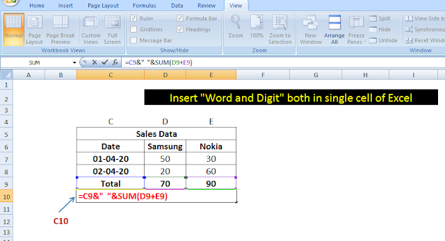
One of the most common tasks is joining text from different cells. The CONCATENATE function does this, but using the ampersand (&) symbol is quicker and more common.
Imagine you have a first name in cell A2 and a last name in B2. To combine them into a full name in C2, you can use:
=A2 & " " & B2
The " " in the middle adds a space between the names. Without it, the result would be "JohnSmith" instead of "John Smith".
Sometimes you need to extract a piece of text from a cell. The LEFT and RIGHT functions are perfect for this.
LEFTextracts a specific number of characters from the beginning of a text string.RIGHTextracts a specific number of characters from the end of a text string.
If cell A2 contains the product code "PROD-12345", you can pull out the text portion or the number portion easily.
// To get the 'PROD' part
=LEFT(A2, 4)

// To get the '12345' part
=RIGHT(A2, 5)
These functions are essential when you need to standardize messy data or prepare it for analysis.
A student's score is in cell A1. To pass, they need a score of 70 or higher. Which formula correctly outputs "Pass" or "Fail"?
To qualify for a promotion, an employee must have sales greater than $50,000 (cell B2) AND a performance rating of at least 4 (cell C2). Which function is most appropriate to check if both conditions are met within a single IF statement?
Mastering these functions will dramatically increase your efficiency and allow you to tackle more complex data challenges in Excel.