Excel Financial Modeling Mastery
Excel Basics
Finding Your Way Around
Opening Excel for the first time can feel like looking at a blank canvas. Let's break down the main parts so you know what you're working with. The main area is a grid of cells, organized into columns (labeled A, B, C...) and rows (labeled 1, 2, 3...). Each cell has a unique address, like A1 or C5. This is where you'll enter your data and formulas.
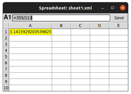
Above the grid, you'll see the Formula Bar. This bar shows the actual content of the selected cell, which is handy because a cell might show a result (like $150) while the formula bar shows the calculation behind it (like =100+50).
At the very top is the Ribbon, which contains all the tools and features organized into tabs like Home, Insert, and Data. Think of it as your toolbox. You'll use it for everything from formatting text to creating charts.
Basic Calculations
Excel is more than just a grid; it's a powerful calculator. You can perform calculations by typing formulas directly into cells. Every formula starts with an equals sign (=).
For simple math, you can type it out directly, like =15*4 to multiply 15 by 4. But the real power comes from using functions to work with your data. Let's say you have a list of monthly sales figures.
| Month | Sales |
|---|---|
| Jan | $1,200 |
| Feb | $1,500 |
| Mar | $1,100 |
To find the total, you don't need to add them manually. You can use the SUM function. If these sales figures were in cells B2, B3, and B4, you'd type this into another cell:
=SUM(B2:B4)
The colon (:) tells Excel to include everything from B2 to B4. Similarly, to find the average monthly sales, you'd use the AVERAGE function:
=AVERAGE(B2:B4)
The IF function lets you make simple decisions. It checks if a condition is true, and then does one thing if it is, and another if it's not. The structure is =IF(condition, value_if_true, value_if_false).
For example, let's say our monthly sales goal is $1,300. We could use IF to see if January (cell B2) met the goal.
=IF(B2>=1300, "Yes", "No")
Since January's sales were $1,200, this formula would display "No".
Keeping Data Tidy
Clear formatting makes your spreadsheet easier to read and understand. You can change numbers to look like currency, percentages, or dates using the tools in the Home tab of the ribbon. A raw number like 0.05 is much clearer when formatted as 5%.
Another way to keep your data clean is Data Validation. This feature lets you set rules for what can be entered into a cell. It's a great way to prevent typos and other errors before they happen.
For instance, you could set a rule that a cell for "Units Sold" must contain a whole number greater than zero. If someone tries to enter -5 or "abc", Excel will show an error message. This ensures the data you're working with is accurate.
Use Data Validation to create dropdown lists. This limits choices to a predefined set, like a list of regions or product names, which is perfect for maintaining consistency.
The Key to Scaling: Cell References
Imagine you have a long list of items and you want to perform the same calculation on each one. You don't need to write a new formula for every row. This is where cell referencing comes in.
By default, Excel uses relative references. This means when you copy a formula down a column, the cell references in the formula automatically adjust. If your formula in C2 is =A2+B2, and you drag it down to C3, the formula will automatically become =A3+B3. It's like giving directions: "add the two cells to my left."
But sometimes you want a reference to stay put. This is called an absolute reference. You create one by adding dollar signs ($) before the column letter and row number, like $A$1.
Let's say you have a list of product prices and a single cell, E1, that contains a sales tax rate of 7%. To calculate the sales tax for each product, you'd use a mix of relative and absolute references.
| A | B | E | |
|---|---|---|---|
| 1 | Product | Price | Tax Rate |
| 2 | T-Shirt | $20.00 | 7% |
| 3 | Mug | $12.00 |
In the cell for the T-Shirt's tax, you would write:
=B2*$E$1
When you copy this formula down for the Mug, the B2 will change to B3 (a relative reference), but $E$1 will stay locked (an absolute reference). This way, every product's price is correctly multiplied by the same tax rate. Mastering this concept is crucial for building models that are easy to expand and update.
Visualizing Your Data
Numbers in a grid are useful, but a chart can tell a story at a glance. Excel makes it easy to create basic charts to visualize your data.
To start, just highlight the data you want to plot, including the labels. Then, go to the Insert tab on the ribbon and choose a chart type. For showing sales over time, a line chart is a great choice. To compare sales across different products, a bar chart works well.
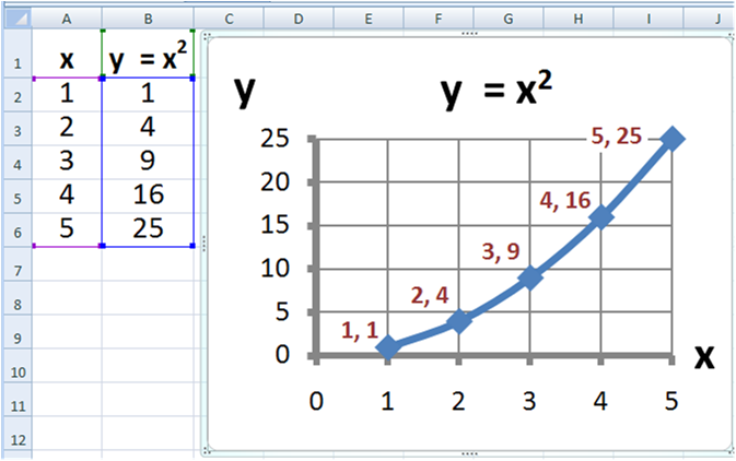
Once the chart is created, you can customize it with titles, axis labels, and different colors to make your message even clearer. Charts are a fundamental tool for communicating the insights you find in your data.
Mastering the basics is the essential first step toward learning advanced data analysis, including pivot tables, VLOOKUP, and macros.
Time to review what you've learned.
In Excel, what is the main purpose of the Formula Bar?
You have a formula in cell C2: =$A2*B$1. If you copy this formula and paste it into cell D3, what will the new formula be?