At its heart, linear algebra is the study of vectors. You can think of a vector as an arrow in space. It has a specific length (magnitude) and points in a specific direction. In data science, we often use vectors to represent a collection of features. For example, a vector could represent a house, with its components being square footage, number of bedrooms, and price.

We usually write vectors as a column of numbers. A vector in a 2D plane, like a computer screen, has two components: one for the x-direction and one for the y-direction.

This vector tells us to go 3 units to the right and 2 units up from the origin (the point (0,0)).

We can perform operations on vectors. Adding two vectors is like placing them tip-to-tail. The new vector, called the resultant, goes from the start of the first vector to the end of the second. Mathematically, we just add the corresponding components.

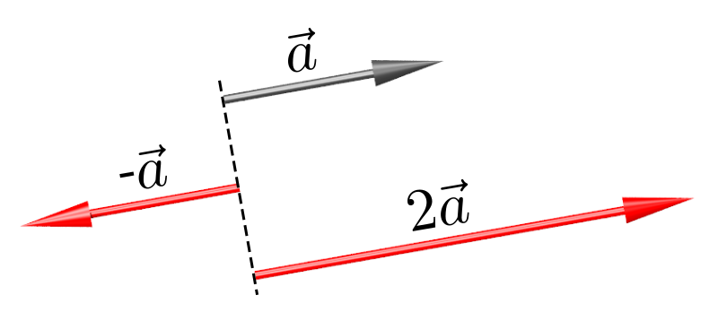
We can also multiply a vector by a single number, called a scalar. This operation scales the vector, making it longer or shorter. Multiplying by a negative scalar flips its direction.

A matrix is a grid of numbers, arranged in rows and columns. You can think of it as a collection of vectors or a way to organize data. For example, a grayscale image is just a matrix where each number represents the brightness of a pixel.

Like vectors, we can perform operations on matrices. Adding two matrices is straightforward: you just add the corresponding elements. This only works if the matrices have the exact same dimensions (the same number of rows and columns).

Matrix multiplication is more involved. To find the element in the first row and first column of the resulting matrix, you take the first row of the first matrix and the first column of the second matrix. You multiply their corresponding elements and then sum the results. This is repeated for every row and column combination.

An important rule for matrix multiplication is that the number of columns in the first matrix must equal the number of rows in the second matrix. Also, unlike regular number multiplication, the order matters. In general, $A \times B$ is not the same as $B \times A$.

So, why are matrices so useful? One of their primary roles is to describe linear transformations. A transformation is just a function that takes an input vector and spits out an output vector. When you multiply a matrix by a vector, you are transforming that vector—rotating it, stretching it, shearing it, or some combination of these.

When we apply a transformation to a vector space, most vectors get knocked off their original direction. But some special vectors are only stretched or shrunk by the transformation; their direction remains unchanged. These are called eigenvectors. The factor by which they are stretched or shrunk is their corresponding eigenvalue.

This relationship is captured by a famous equation where $A$ is the matrix, $\vec{v}$ is the eigenvector, and $\lambda$ (the Greek letter lambda) is the eigenvalue.

This equation says that transforming the vector $\vec{v}$ with matrix $A$ has the same effect as just scaling it by the number $\lambda$. Eigenvectors and eigenvalues reveal deep properties of a matrix and are fundamental to many algorithms in data science, like Principal Component Analysis (PCA) for dimensionality reduction.