Diffusion Transformers Explained
Introduction to Diffusion Models
Sculpting from Static
Imagine a sculptor who doesn't start with a block of marble, but with a cloud of dust. Instead of chipping material away, they carefully guide the dust particles to settle and form a detailed statue. This is the core idea behind diffusion models, a powerful type of generative AI.
Diffusion models create new data, such as images or audio, by transforming random noise into a coherent result through a step-by-step process.
This method has become the engine behind many state-of-the-art image generators. The magic lies in a two-part process: first, learning how to destroy an image, and then, using that knowledge to create a new one from scratch.
The Forward and Reverse Processes
The entire concept of diffusion models is built on two opposite journeys: the forward process and the reverse process.
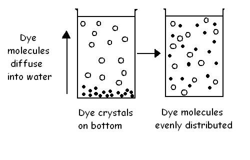
The forward process is the destructive part. It takes a perfectly clear image and gradually adds a tiny bit of random, Gaussian noise at each step. This continues for hundreds or thousands of steps until the original image is completely lost in a sea of static. This process is fixed; it doesn't involve any 'learning.' We define exactly how much noise to add at each step.
The reverse process is where the learning happens. The AI model is trained to do the exact opposite. It starts with a field of pure noise and, step-by-step, removes just the right amount of noise to slowly reveal a clear, new image. To do this, at every step, the model must predict the noise that was added in the forward process so it can subtract it.
Data generation is achieved using a learnt, parametrized reverse process that performs iterative denoising, starting from pure random noise (see figure above).
A Look at the Math
Let's peek under the hood, without getting too complicated. Let be our original, clean image. The forward process at each step creates a slightly noisier image, , from the previous one, .
This is done by adding a small amount of Gaussian noise, controlled by a value . The formula looks like this:
Here, slightly shrinks the previous image's data, and adds in the new noise. After many steps, all that's left is noise. This sequence of values, known as the variance schedule, determines how quickly the image dissolves into static.
The model's goal in the reverse process is to learn the reverse of this. It needs to predict the noise that was added to to get back to a cleaner . In essence, it learns a function that estimates the noise in the image at step .
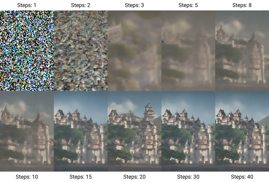
By repeatedly predicting and subtracting this noise, the model can navigate backward from pure static to a brand new, coherent image.
This unique approach of destroying and then recreating data is what allows diffusion models to generate such diverse and high-quality results. They are used in creating images, generating audio, modeling 3D shapes, and even in scientific fields like drug discovery. By mastering a simple process of adding noise, these models learn the complex task of creation.