Data Science Professional Pathway
Complex Data Wrangling
Beyond Basic Queries
You already know how to pull data with SELECT and join tables. But real-world datasets are rarely that simple. They're tangled webs of events over time, requiring more than basic queries to make sense of them. Instead of pulling massive, raw tables into Python and wrestling with them there, we can perform sophisticated data shaping directly in the database. This saves time, memory, and a lot of headaches.
Two powerful tools for this are window functions and Common Table Expressions (CTEs). Window functions let you perform calculations across a set of rows related to the current row, like calculating a running total or ranking sales within a category. They're your key to analyzing sequences and trends without complex self-joins.
Common Table Expressions are like temporary, named result sets that you can reference within a larger query. Think of them as building blocks. You can define one CTE to clean your data, another to aggregate it, and then join them together in a final, clean SELECT statement. This makes long, complicated queries readable and easier to debug.
WITH UserLoginHistory AS (
  SELECT
    user_id,
    login_timestamp,
    -- The LAG function looks back 1 row within this user's login history
    LAG(login_timestamp, 1) OVER (PARTITION BY user_id ORDER BY login_timestamp) AS previous_login
  FROM logins
)
SELECT
  user_id,
  login_timestamp,
  previous_login,
  -- Calculate the time difference between consecutive logins
  JULIANDAY(login_timestamp) - JULIANDAY(previous_login) AS days_since_last_login
FROM UserLoginHistory
WHERE previous_login IS NOT NULL; -- Exclude the very first login for each user
This query uses a CTE named UserLoginHistory to create a temporary table. Inside it, the LAG window function finds each user's previous login time. The final SELECT statement then uses this temporary table to calculate the time between consecutive logins. Trying to do this with a standard JOIN would be far more complicated.
Wrangling Data at Scale
Once data is in Python, performance becomes critical, especially with datasets containing millions of rows. The default approach for many is to loop through a Pandas DataFrame, but this is incredibly slow. The key to speed is vectorized operations with NumPy and Pandas. These libraries perform operations on entire arrays of data at once, using highly optimized, low-level code (often written in C or Fortran). Instead of processing one element at a time, you apply a function to the whole column.
Memory management is another challenge. A DataFrame with millions of rows can easily consume all your available RAM. One effective strategy is to downcast data types. For instance, if a column of integers only contains values up to 100, you don't need a 64-bit integer (int64) to store it; an 8-bit integer (int8) will do, using 8 times less memory. Pandas has tools to help you analyze and convert columns to their most memory-efficient types.
import pandas as pd
import numpy as np

# Create a large DataFrame to simulate real data
df = pd.DataFrame({
    'temperature': np.random.uniform(15.0, 30.0, 1_000_000),
    'humidity': np.random.uniform(40.0, 80.0, 1_000_000)
})

# --- NON-VECTORIZED (SLOW) ---
def celsius_to_fahrenheit_loop(temps):
    fahrenheit_temps = []
    for temp in temps:
        fahrenheit_temps.append((temp * 9/5) + 32)
    return fahrenheit_temps

# %timeit df['fahrenheit_loop'] = celsius_to_fahrenheit_loop(df['temperature'])
# This would be very slow on a large dataset.

# --- VECTORIZED (FAST) ---
# The operation is applied to the entire series at once.
df['fahrenheit_vectorized'] = (df['temperature'] * 9/5) + 32
The vectorized approach is not just cleaner to write; it can be orders of magnitude faster. Always look for ways to apply operations to entire columns or arrays instead of iterating.
Automated Cleaning and Imputation
Real data is messy. It's full of missing values, typos, and outliers that can skew your analysis. While you can manually fix a few issues, production data pipelines need automated, robust methods for cleaning.
For detecting anomalies, simple statistical rules (like flagging anything beyond three standard deviations) can fail with complex data. A more advanced technique is the Isolation Forest algorithm. It works by randomly partitioning the data, effectively isolating outliers in just a few steps. It's efficient and doesn't rely on assumptions about the data's distribution.
Handling missing data is another critical step. Simply dropping rows with missing values can discard valuable information, and filling them with the mean or median is often too simplistic. More sophisticated imputation methods like k-Nearest Neighbors (k-NN) or MICE (Multivariate Imputation by Chained Equations) can provide more accurate estimates. k-NN finds the 'k' most similar complete rows and uses their values to impute the missing one. MICE builds a model to predict the missing values based on all the other columns, treating each column with missing data as the target in a series of regressions.
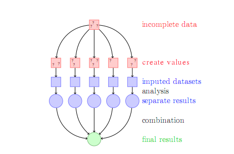
Choosing the right imputation method depends on the nature of your data. If values are missing completely at random, simpler methods might suffice. But if the missingness is related to other variables, a model-based approach like MICE is generally superior.
Data Cleaning: Learn how to clean and preprocess messy datasets, which is often 80% of the work in data science projects.
Now let's test your understanding of these advanced wrangling techniques.
What is a primary advantage of using Common Table Expressions (CTEs) and window functions directly in a database query?
When processing a large Pandas DataFrame, why are vectorized operations (e.g., df['column'] * 2) superior to iterating with a for loop?
Mastering these techniques for shaping, cleaning, and efficiently processing data is what separates basic analysis from production-ready data science. It's the critical foundation for any reliable model.