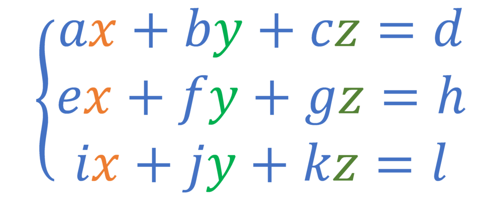
Solving a system of linear equations is about finding the specific point where multiple lines or planes intersect. For a simple case with two variables, you might find a unique solution, no solution if the lines are parallel, or infinite solutions if they're the same line. As you add more variables and equations, visualizing this becomes difficult, but the underlying principles remain the same.

The first step is to stop thinking about the variables themselves and focus on the coefficients. We can represent a system of equations as an augmented matrix. This strips away the variables like $x$, $y$, and $z$, leaving just the numbers in a structured grid.

Working with this matrix is much cleaner. Our goal is to manipulate it using a systematic process called Gaussian elimination to make the solution obvious. This process relies on three simple, allowed operations:

1. Swapping two rows.
2. Multiplying a row by a non-zero constant.
3. Adding a multiple of one row to another row.

The immediate goal of Gaussian elimination is to get the matrix into Row Echelon Form (REF). A matrix is in REF if it satisfies two conditions:

• All rows consisting entirely of zeros are at the bottom.
• The first non-zero number from the left in each row, called the pivot, is to the right of the pivot of the row above it.

This creates a staircase-like pattern of zeros in the bottom-left corner of the matrix. Let's apply this to our example. The first pivot is already a 1 in the top-left, which is convenient. Our first step is to create zeros below it.

We subtract 2 times the first row from the second, and 3 times the first row from the third. Now our pivot for the second row is -5. We can simplify this row by dividing it by -5.

Finally, we use our new second row to create a zero below its pivot. We add 6 times the second row to the third row.

This matrix is in REF. From here, we can use a technique called back-substitution. We convert the matrix back into equations:

• $-4z = -12$
• $y + z = 2$
• $x + 2y + 3z = 9$

Solving the first equation gives $z=3$. Plugging that into the second gives $y + 3 = 2$, so $y=-1$. Plugging both into the top equation gives $x + 2(-1) + 3(3) = 9$, which simplifies to $x - 2 + 9 = 9$, so $x=2$. The unique solution is $(2, -1, 3)$.

Back-substitution is effective, but it's still a manual process. We can continue the elimination algorithm to simplify the matrix even further, to a state called Reduced Row Echelon Form (RREF). This form has two additional rules:

• Every pivot is 1.
• Each pivot is the only non-zero entry in its column.

This process is called Gauss-Jordan reduction. Starting from our REF matrix, we first make the last pivot a 1 by dividing the last row by -4.

Now, we work backwards from the bottom-right pivot to create zeros above it. We subtract the third row from the second, and 3 times the third row from the first.

One final step: use the second row's pivot to eliminate the 2 above it. We subtract 2 times the second row from the first.

Now, converting back to equations is trivial: $x = 2$, $y = -1$, and $z = 3$. The solution is read directly from the final column. For any given matrix, its RREF is unique, making it a powerful canonical form for analyzing systems.

The positions of the pivots tell us everything about the nature of the solution. The columns that contain a pivot are called pivot columns. The variables corresponding to these columns are basic variables. In our example, all three variables ($x, y, z$) were basic variables, which led to a single, unique solution.

But what if a column lacks a pivot? Such a column corresponds to a free variable. This means the variable can take on any value, and we can express the other (basic) variables in terms of it. This occurs when there are fewer independent equations than variables, resulting in infinitely many solutions.

Consider a system that reduces to this RREF:

Here, $x$ and $y$ are basic variables, but $z$ is a free variable. The last row, $0=0$, is consistent but provides no information. The other rows give us:

• $x - 2z = 5 \tRightarrow x = 5 + 2z$
• $y + 4z = -1 \tRightarrow y = -1 - 4z$

We can pick any value for $z$ (say, $z=t$) and find a corresponding $x$ and $y$. The solution set is a line in 3D space described by the vector $(5, -1, 0) + t(2, -4, 1)$ for any real number $t$.

The set of all solutions to the homogeneous equation $A\vec{x} = \vec{0}$ (where the constant terms are all zero) forms a vector space called the null space or kernel of the matrix $A$. The number of free variables in the echelon form of $A$ corresponds to the dimension of this null space. This leads to a foundational result in linear algebra.

This theorem provides a deep connection between the structure of a matrix and the solution space of the linear system it represents. Understanding this structure is the computational key to finding eigenvectors and exploring other advanced topics.

Ready to test your understanding?

Mastering this algorithmic approach is essential. It transforms messy systems of equations into a standardized form where the nature of the solution becomes clear.