In the world of complex functions, not all points are created equal. While many points behave predictably, some are special. These are the points where a function might shoot off to infinity, or become otherwise undefined. We call these points singularities.

A singularity of a function $f(z)$ is a point $z_0$ where the function is not analytic. For our purposes, we're interested in isolated singularities, where the function is analytic in a small neighbourhood around the point, just not at the point itself.

There are three main types of isolated singularities:

1. Removable Singularities: These are like potholes that can be filled. The function might not be defined at the point, but we can assign a value to it to make the function analytic there. For example, the function $f(z) = \frac{\sin(z)}{z}$ is undefined at $z=0$, but its limit as $z \to 0$ is 1. We can just define $f(0)=1$ and the problem is solved.
2. Poles: These are more serious. At a pole, the function's magnitude blows up to infinity. Think of the function $f(z) = \frac{1}{z-2}$. At $z=2$, the denominator is zero, and the function's value is infinite. This is a pole.
3. Essential Singularities: These are the most complex. As you approach an essential singularity, the function behaves erratically, taking on every possible complex value (with at most one exception) in any tiny neighbourhood around the point. The function $f(z) = e^{1/z}$ has an essential singularity at $z=0$.

Poles are particularly important in engineering applications, especially when solving integrals. They are classified by their order. A pole at $z_0$ is of order $n$ if the function $f(z)$ can be written in a specific form. Intuitively, the order tells you "how fast" the function goes to infinity. A pole of order 2 goes to infinity faster than a pole of order 1.

For a function $f(z)$ to have a pole of order $n$ at $z_0$, the function $\phi(z) = (z-z_0)^n f(z)$ must be analytic and non-zero at $z_0$. The simplest case is a simple pole, where the order is $n=1$.

Around any isolated singularity, we can express a function using a Laurent series, which is like a Taylor series but can also include terms with negative powers. The Laurent series for a function $f(z)$ about a point $z_0$ looks like this:

$f(z) = \sum_{k=-\infty}^{\infty} a_k (z-z_0)^k = \dots + \frac{a_{-2}}{(z-z_0)^2} + \frac{a_{-1}}{z-z_0} + a_0 + a_1(z-z_0) + \dots$

One of these coefficients is uniquely important: the coefficient $a_{-1}$. This is called the residue of the function $f(z)$ at the singularity $z_0$. It's often denoted as $\text{Res}(f, z_0)$.

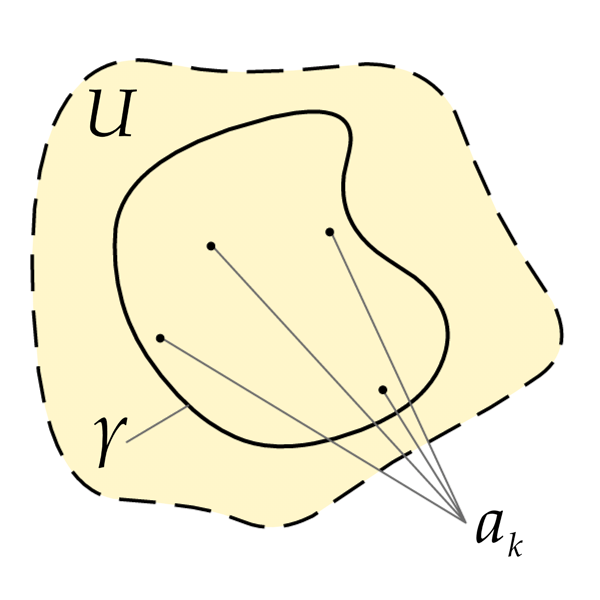
The residue might seem like just one of many numbers, but it holds the key to evaluating many complex integrals that are otherwise intractable. The Residue Theorem, which you'll see later, uses the sum of residues inside a closed path to calculate the integral along that path.

Finding the full Laurent series just to get one coefficient can be tedious. Thankfully, we have more direct methods for calculating residues at poles.

For a simple pole ($n=1$), the calculation is straightforward. You can find the residue by multiplying the function by $(z-z_0)$ and then taking the limit as $z$ approaches $z_0$.

Let's find the residue of $f(z) = \frac{e^z}{z-i}$ at its pole $z_0=i$.

For a pole of order n, the formula is a bit more involved. It requires taking a derivative to isolate the $a_{-1}$ coefficient.

For example, consider $f(z) = \frac{z}{(z-3)^2}$. This has a pole of order 2 at $z_0=3$. Here, $n=2$.

Sometimes, the limit formulas are cumbersome, especially if the function is complex. In these cases, it can be easier to find the first few terms of the Laurent series expansion and simply read off the $a_{-1}$ coefficient.

For example, to find the residue of $f(z) = \frac{\cos(z)}{z^3}$ at $z=0$, we can use the known series for $\cos(z)$.

From the expansion, we can see that the coefficient of the $\frac{1}{z}$ term is $-\frac{1}{2}$. So, $\text{Res}(f, 0) = -1/2$.

Understanding how to identify singularities and calculate their residues is a foundational skill for applying complex analysis to practical problems.