Choosing Classification Metrics
Confusion Matrix
Beyond Simple Accuracy
When we build a model to classify things—like telling spam emails from real ones—we need a way to measure how well it's doing. A simple accuracy score, like "85% correct," can be misleading. It doesn't tell us about the types of mistakes the model is making. Is it letting spam into our inbox, or is it sending important emails to the spam folder? To get this deeper insight, we use a tool called a confusion matrix.
A confusion matrix is a simple table that breaks down a model's performance. It compares the model’s predictions against the actual, real-world outcomes. This comparison helps us see exactly where the model is succeeding and where it's getting confused.
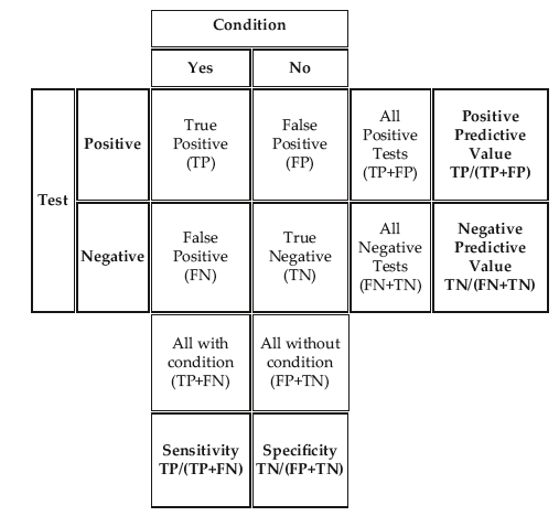
The matrix has four cells, each representing one of four possible outcomes for any prediction.
The Four Outcomes
Let's imagine a model that predicts whether an email is spam. The "positive" class is "spam," and the "negative" class is "not spam."
Every prediction the model makes will fall into one of these four categories:
True Positive (TP): The model correctly predicts the positive class. It sees a spam email and correctly labels it as spam.
True Negative (TN): The model correctly predicts the negative class. It sees a normal email and correctly labels it as not spam.
False Positive (FP): The model incorrectly predicts the positive class. It sees a normal email but mistakenly labels it as spam. This is also known as a Type I error.
False Negative (FN): The model incorrectly predicts the negative class. It sees a spam email but mistakenly labels it as not spam, letting it into your inbox. This is a Type II error.
The terms "true" and "false" tell you if the model was right or wrong. The terms "positive" and "negative" refer to what the model predicted.
Calculating Accuracy
With these four values, we can calculate the overall accuracy of the model. Accuracy measures the proportion of total predictions that were correct. To find it, we add the correct predictions (TP and TN) and divide by the total number of predictions (all four categories combined).
Let's use our spam filter example. Suppose we test it on 1000 emails. Here are the results:
- True Positives (TP): 130 (130 spam emails were correctly identified)
- True Negatives (TN): 810 (810 normal emails were correctly identified)
- False Positives (FP): 20 (20 normal emails were flagged as spam)
- False Negatives (FN): 40 (40 spam emails were missed)
Now, let's plug these numbers into the formula:
The model's accuracy is 94%. This seems high, but the confusion matrix gives us a much richer story. It tells us that while the model is mostly accurate, it still missed 40 spam emails and incorrectly blocked 20 legitimate ones. Depending on the situation, these errors could be very important.
And that's the power of the confusion matrix. It moves us beyond a single number and gives us the context we need to truly evaluate a model's performance.