Calculus-Based Statistics Foundations
Random Variables
Numbers from Chance
Many things in life are uncertain. Will it rain tomorrow? Will my favorite team win? Will the bus be on time? Probability helps us reason about this uncertainty, but it's often useful to attach numbers to the outcomes of these random events.
This is where random variables come in. A random variable is a way to map the outcomes of a random process to numbers. It’s a variable, but its value is determined by chance.
Imagine you flip a coin. The outcomes are 'Heads' or 'Tails'. We can define a random variable, let's call it , where if the coin is Heads, and if it's Tails. The variable now numerically represents the coin flip's result.
Random Variable
noun
A function that assigns a numerical value to each possible outcome of a random experiment.
By converting outcomes into numbers, we can use the tools of mathematics to analyze them. We can calculate averages, find the spread of the data, and model real-world phenomena. But not all random variables are the same. They fall into two main categories: discrete and continuous.
Countable vs. Measurable
The distinction between discrete and continuous random variables is fundamental. It all comes down to the types of numbers they can represent.
Clearly distinguish between discrete and continuous variables since the approach to probability calculations differs significantly.
A discrete random variable takes on a countable number of distinct values. Think of things you can count, like the number of cars passing a point in an hour, or the number of heads in four coin flips. The values are separate and distinct, like 0, 1, 2, 3, and so on.
For each possible value of a discrete random variable, we can assign a probability. This set of probabilities is called a Probability Mass Function, or PMF. The PMF tells us the probability that the random variable is exactly equal to some value . We write this as .
A key property of a PMF is that if you add up the probabilities for all possible values, the sum is always 1. This makes sense, because one of the outcomes must occur.
| Roll () | Probability |
|---|---|
| 1 | 1/6 |
| 2 | 1/6 |
| 3 | 1/6 |
| 4 | 1/6 |
| 5 | 1/6 |
| 6 | 1/6 |
The table above shows the PMF for a single roll of a fair six-sided die. The probability of rolling any specific number is exactly 1/6. If we sum the probabilities: $1/6 + 1/6 + 1/6 + 1/6 + 1/6 + 1/6 = 1$.
A continuous random variable, on the other hand, can take on any value within a given range. Think of things you measure, like the height of a person, the temperature of a room, or the exact time it takes to run a mile. For any two values in the range, there's an infinite number of other possible values between them.
Here's a tricky part: for a continuous random variable, the probability of it being exactly a specific value is zero. Why? Because there are infinitely many possible values. It's like trying to hit a single, infinitesimally small point on a line with a dart. The chances are zero.
Instead, we talk about the probability of the variable falling within a range of values. We do this using a Probability Density Function, or PDF, usually written as $f(x)$. The PDF itself is not a probability, but the area under its curve between two points gives the probability that the variable will fall in that interval.
Like a PMF, the total area under the curve of a PDF must equal 1, representing the certainty that the value will fall somewhere within its possible range.
The Cumulative Story
Sometimes we don't care about the probability of a single outcome or a specific range. Instead, we want to know the probability that our random variable is less than or equal to a certain value. This is where the Cumulative Distribution Function, or CDF, comes in.
The CDF, written as , gives the probability . It
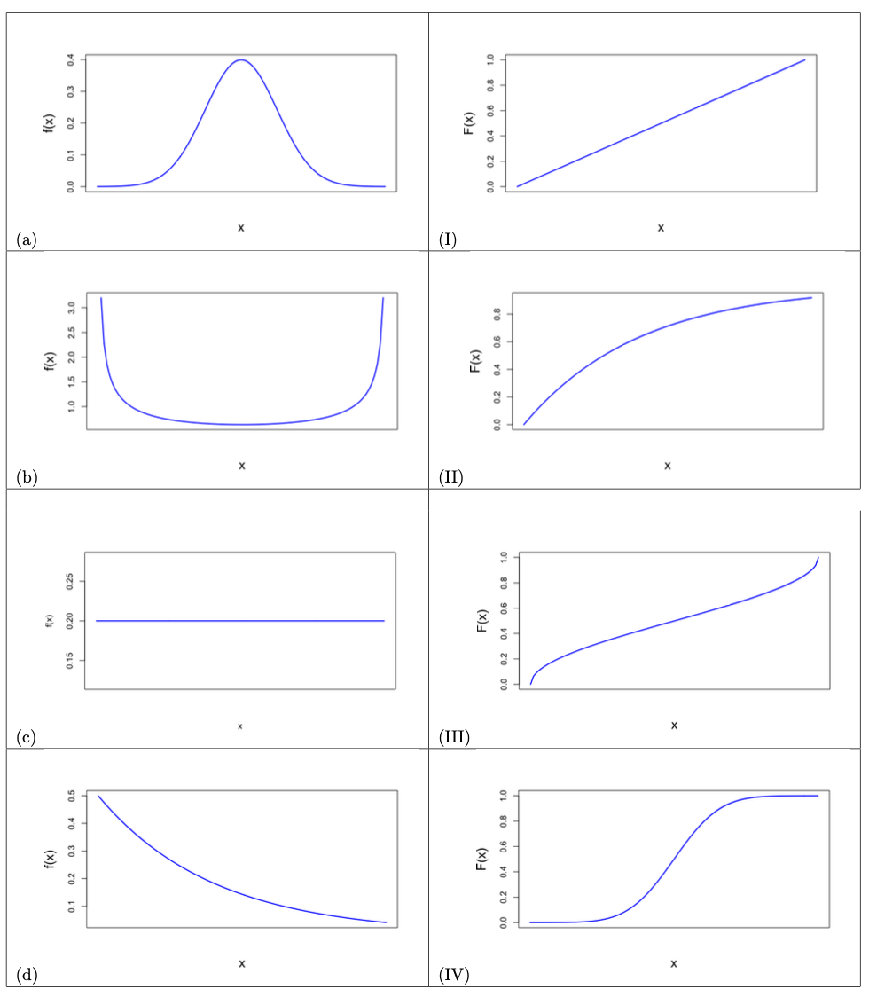
Notice a few key properties from these graphs. The CDF always starts at 0 (or approaches it) on the far left and ends at 1 (or approaches it) on the far right. This is because the probability of being less than some very small number is 0, and the probability of it being less than some very large number is 1.
Also, the CDF is always non-decreasing. As you move from left to right along the x-axis, the cumulative probability can only stay the same or increase. It can never go down.
For a discrete variable, the CDF is a step function—it jumps up at each possible value. For a continuous variable, the CDF is a smooth, continuous curve. It is the integral of the PDF.
The CDF is incredibly useful because it unifies the concepts for both discrete and continuous variables. It provides a complete description of the probability distribution of a random variable.
What is the primary purpose of a random variable?
Which of the following is an example of a discrete random variable?
Understanding these foundational concepts is the first step toward using probability to model and understand the complex, random world around us.