Building Machine Learning from the Ground Up
Matrix Operations and Data
Data as Arrays
In machine learning, data is represented numerically. Whether it's pixel values from an image, word counts from a document, or user ratings for a movie, everything gets converted into arrays of numbers. A single data point, like an image, can be a vector. A collection of data points becomes a matrix, and a sequence of matrices, like in video data, becomes a higher-dimensional tensor. For all of this, Python's go-to library is NumPy.
NumPy provides the ndarray object, a powerful N-dimensional array that is far more efficient for numerical operations than standard Python lists. Because you're already familiar with Python, we'll skip the basics and jump right into how these arrays form the bedrock of ML algorithms.
import numpy as np

# A matrix representing 3 data points, each with 4 features.
# Think of it as 3 users and their scores on 4 different metrics.
data = np.array([
    [10, 8, 12, 9],
    [5, 4, 6, 5],
    [22, 18, 25, 20]
])

print(data.shape)
# Output: (3, 4)
Core Operations
Two fundamental matrix operations you'll use constantly are the dot product and transposition. The dot product is the engine of many ML models, especially neural networks, where it's used to calculate the weighted sum of inputs. It combines two matrices into a new one, but only if their inner dimensions match. For example, you can multiply a (3, 4) matrix by a (4, 2) matrix, resulting in a (3, 2) matrix. The '4's in the middle align.
# Let's define a weight matrix.
# This could represent the weights of a simple neural network layer.
# It has 4 rows to match the 4 features of our data, and 2 columns for 2 output neurons.
weights = np.array([
    [0.1, 0.5],
    [-0.2, 0.3],
    [0.4, -0.6],
    [-0.3, 0.1]
])

# Calculate the dot product
# The @ operator is a convenient shorthand for np.dot()
output = data @ weights

print(output.shape)
# Output: (3, 2)

print(output)
# [[1.5, 3.8],
#  [0.7, 2.8],
#  [4.4, 7.8]]
Transposition flips a matrix over its diagonal. It swaps the row and column indices. This is often a simple but necessary mechanical step to make sure the dimensions of two matrices are compatible for multiplication.
# Let's say we have a (2, 3) matrix
A = np.array([
    [1, 2, 3],
    [4, 5, 6]
])

# Its transpose will be a (3, 2) matrix
A_transposed = A.T

print(A_transposed)
# [[1, 4],
#  [2, 5],
#  [3, 6]]
Broadcasting and Vectorization
Imagine you want to add a bias value to each of the outputs we calculated earlier. You could write a loop, but that's slow in Python. NumPy provides a much faster, more elegant solution called broadcasting.
Broadcasting describes how NumPy treats arrays with different shapes during arithmetic operations. Subject to certain constraints, the smaller array is "broadcast" across the larger array so that they have compatible shapes. This allows you to perform operations between a large array and a small one without making explicit copies of the small array. This principle is part of a larger concept called Vectorization—writing code that operates on entire arrays at once instead of individual elements.
# `output` is our (3, 2) matrix from before
# `bias` is a (1, 2) vector
bias = np.array([0.1, -0.2])

# NumPy automatically "stretches" or broadcasts the bias vector
# to be added to each of the three rows in `output`.
final_output = output + bias

print(final_output)
# [[1.6, 3.6],
#  [0.8, 2.6],
#  [4.5, 7.6]]
Preparing Data for Models
Raw data rarely comes in a clean, model-ready format. One of the most important preprocessing steps is feature scaling. Many ML algorithms, particularly those using gradient-based optimization like linear regression and neural networks, perform better when input features are on a similar scale. If one feature ranges from 0 to 1 and another from 0 to 1,000,000, the algorithm may become unstable and struggle to find the optimal solution.
Two common scaling techniques are normalization and standardization.
Normalization scales data to a fixed range, usually 0 to 1. This is also known as min-max scaling.
def normalize(data):
    """Scales data to the [0, 1] range."""
    min_vals = data.min(axis=0) # Find min of each column (feature)
    max_vals = data.max(axis=0) # Find max of each column
    return (data - min_vals) / (max_vals - min_vals)

normalized_data = normalize(data)
print(normalized_data)
Standardization scales data to have a mean of 0 and a standard deviation of 1. It does not bound values to a specific range.
def standardize(data):
    """Scales data to have a mean of 0 and a standard deviation of 1."""
    mean_vals = data.mean(axis=0)
    std_devs = data.std(axis=0)
    return (data - mean_vals) / std_devs

standardized_data = standardize(data)
print(standardized_data)
Splitting the Data
Finally, to evaluate a model's performance, we can't test it on the same data we used for training. That would be like giving a student an exam with the exact questions they studied—it doesn't prove they learned the concepts, only that they memorized the answers. We need to split our dataset into a training set and a test set. The model learns from the training set, and its ability to generalize to new, unseen data is measured on the test set.
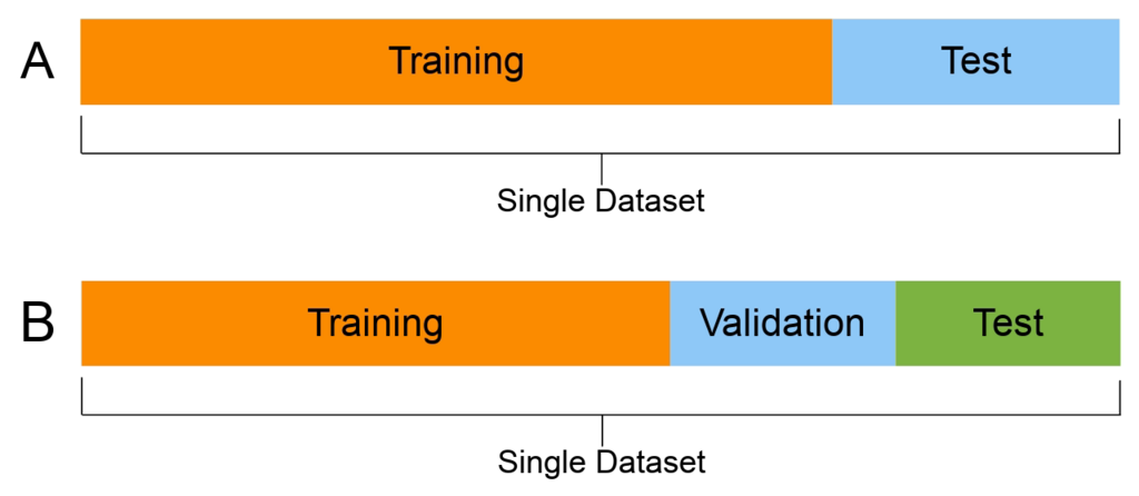
The logic is straightforward: shuffle the data to remove any order bias, then slice it into two pieces. A common split is 80% for training and 20% for testing.
def split_data(X, y, test_size=0.2):
    """Splits features (X) and labels (y) into train and test sets."""
    # Create a shuffled list of indices
    num_samples = X.shape[0]
    indices = np.arange(num_samples)
    np.random.shuffle(indices)

    # Determine the split point
    split_idx = int(num_samples * (1 - test_size))

    # Slice the data using the shuffled indices
    train_indices, test_indices = indices[:split_idx], indices[split_idx:]

    X_train, X_test = X[train_indices], X[test_indices]
    y_train, y_test = y[train_indices], y[test_indices]

    return X_train, X_test, y_train, y_test

# Example usage:
# Assume `labels` is a corresponding vector for our `data` matrix
labels = np.array([1, 0, 1])

X_train, X_test, y_train, y_test = split_data(data, labels)

print(f"X_train shape: {X_train.shape}")
print(f"X_test shape: {X_test.shape}")
These NumPy operations—multiplication, broadcasting, scaling, and splitting—are the essential mechanics you'll use to build, train, and evaluate virtually every machine learning model.