Bayesian Econometrics Essentials
Bayesian Basics
Thinking in Probabilities
How do we learn? We start with an idea about how the world works, and as we encounter new information, we adjust our beliefs. If you think it rarely rains in the desert, but you see dark clouds gathering, you might update your belief and grab an umbrella. This process of updating beliefs in the face of new evidence is the core idea behind Bayesian statistics.
Bayesian thinking is a way to formally combine existing knowledge with new evidence.
Instead of treating probabilities as fixed, long-run frequencies of events, the Bayesian approach treats probability as a measure of our certainty or belief about something. This perspective is incredibly powerful because it gives us a mathematical way to get less wrong over time.
The Core Idea: Bayes' Theorem
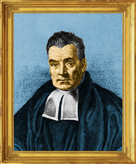
The engine that drives this process is a surprisingly simple formula called Bayes' theorem. It was developed by Thomas Bayes, an 18th-century statistician and minister. The theorem tells us exactly how to update our belief about a hypothesis when we get new data.
Let's say our hypothesis is 'A' and the new evidence is 'B'. Bayes' theorem connects the probability of A given B to the probability of B given A. The formula looks like this:
It might look intimidating, but each part has a specific name and a clear role. Let's break it down.
Posterior
noun
This is what we're trying to find: P(A|B), the probability of our hypothesis A being true, given the new evidence B. It's our updated belief after seeing the data.
The posterior belief is calculated from two main ingredients: our initial belief and the new evidence.
Prior
noun
This is our initial belief about the hypothesis: P(A). It's the probability we assign to A before we see any new evidence. This is our starting point.
Likelihood
noun
This represents the new evidence: P(B|A). It's the probability of observing the evidence B if our hypothesis A were true. It links our data to our hypothesis.
The term on the bottom, , is the overall probability of observing the evidence. It acts as a normalizing constant, ensuring the final posterior probability is on a scale from 0 to 1.
So, the formula can be summarized in words:
Posterior Belief = (Likelihood of Evidence × Prior Belief) / Total Probability of Evidence
Bayes’ Theorem highlights the importance of updating your estimates in light of new evidence.
Updating Beliefs in Action
Let’s use a classic example. Imagine a rare disease that affects 1 in 1,000 people (0.1%). There’s a test for this disease that is 99% accurate. This means it correctly identifies 99% of people who have the disease (true positive) and correctly identifies 99% of people who don't (true negative).
You take the test and it comes back positive. What is the probability that you actually have the disease?
Our intuition might scream 99%, but let's use Bayes' theorem to find out. Let's define our terms:
- A: You have the disease.
- B: You test positive.
We want to find , the probability you have the disease given a positive test.
Our prior, , is our belief before the test: 1/1000 or 0.001. Our likelihood, , is the probability of testing positive if you have the disease: 0.99 (the test's accuracy).
The trickiest part is calculating , the total probability of testing positive. A person can test positive in two ways: they have the disease and test positive (a true positive), or they don't have the disease and test positive (a false positive).
- Probability of a true positive:
- Probability of a false positive: The test has a 1% error rate for healthy people (1 - 0.99 = 0.01). The probability of not having the disease is . So, .
The total probability of testing positive, , is the sum of these two scenarios: .
Now we can plug everything into Bayes' theorem:
Surprisingly, even with a positive result from a 99% accurate test, the probability you actually have the disease is only about 9%! Our initial belief (the prior) was very low because the disease is so rare, and that heavily influenced the outcome. The test result updated our belief, making it much higher than 1 in 1,000, but still far from certain.
Two Flavors of Statistics
This way of thinking marks a key difference between Bayesian and another major school of thought, frequentist statistics. For a frequentist, the probability of an event is its long-run frequency. For example, the probability of a coin landing heads is 0.5 because if you flipped it a huge number of times, it would land heads about half the time. This view works well for things you can repeat, like coin flips, but less so for one-time events, like an election outcome or whether a specific economic theory is true.
A Bayesian, on the other hand, sees probability as a degree of belief. It's a way to quantify our uncertainty. This allows Bayesians to assign probabilities to hypotheses, something a frequentist would not do. A Bayesian can say "there is a 90% probability that I have this disease," while a frequentist would focus on the error rates of the test over many repetitions.
| Feature | Bayesian Approach | Frequentist Approach |
|---|---|---|
| Probability | Degree of belief or confidence | Long-run frequency of an event |
| Parameters | Random variables with probability distributions | Fixed, unknown constants |
| Inference Focus | Posterior distribution of parameters | Point estimates and confidence intervals |
| Key Tool | Bayes' Theorem | p-values, Null Hypothesis Testing |
One of the main advantages of the Bayesian approach is its ability to formally incorporate prior information. If previous studies suggest a certain economic policy is effective, a Bayesian analysis can start with that knowledge as a prior, and then update it with new data. It also provides a full probability distribution for the results, which can offer a richer understanding of uncertainty than a single point estimate and a confidence interval.
Now, let's test your understanding of these foundational concepts.
What is the fundamental principle of the Bayesian approach to statistics?
In Bayes' theorem, , what does the term represent?
Understanding these core ideas—priors, likelihoods, and posteriors—is the first step into the world of Bayesian econometrics, where we can build models that learn from data and quantify our uncertainty about the economic world.