Each Global Navigation Satellite System (GNSS) satellite carries a highly stable atomic clock. However, the raw 'tick' of this clock isn't the time broadcast to Earth. The satellite must first establish its own internal, coherent time scale, known as Satellite Vehicle (SV) time. This process begins by observing the phase of the clock's output signal. This raw signal is the foundation, but it's not perfect. It's affected by noise and environmental factors unique to space.

The goal is to translate the clock's physical oscillations into a stable, predictable time reference. This internal reference is what the satellite uses for its own operations and as the basis for the navigation signals it transmits. Before this time scale can be trusted, its stability must be rigorously characterised.

Standard deviation is useful for many things, but it struggles to describe the stability of an oscillator over different time intervals. Instead, engineers rely on the Allan Variance (AVAR). It's a measure of frequency stability that analyses how the clock's frequency changes as you average it over longer and longer periods, from seconds to hours to days. This is crucial in orbit, where a clock's performance can drift due to temperature changes, radiation, and aging.

By analysing the Allan Variance plot, specific types of clock noise can be identified. These are not random errors in the traditional sense; they are distinct patterns of deviation that give insight into the clock's physical behaviour. Understanding these noise models is the key to predicting and correcting for clock errors.

The raw output of an atomic clock can be modelled as a combination of a perfect time signal and several noise components. The three primary noise types relevant to GNSS are:

• White Phase Modulation (WPM): This is high-frequency jitter, essentially random noise on the phase of the signal. It's most significant over very short time scales.
• White Frequency Modulation (WFM): This is random noise on the frequency itself. It's a key indicator of the clock's short-term stability, often called its 'random walk in phase'.
• Random Walk Frequency Modulation (RWFM): This represents a slow, unpredictable drift in the clock's frequency over long periods. This is often the limiting factor for a clock's long-term stability and is caused by slow changes in the clock's physical components.

Characterising the initial frequency offset ($y_0$) is one of the first and most important steps. It's the constant rate at which the satellite's clock runs slightly faster or slower than the ideal reference time. This offset is measured and forms the basis for initial corrections.

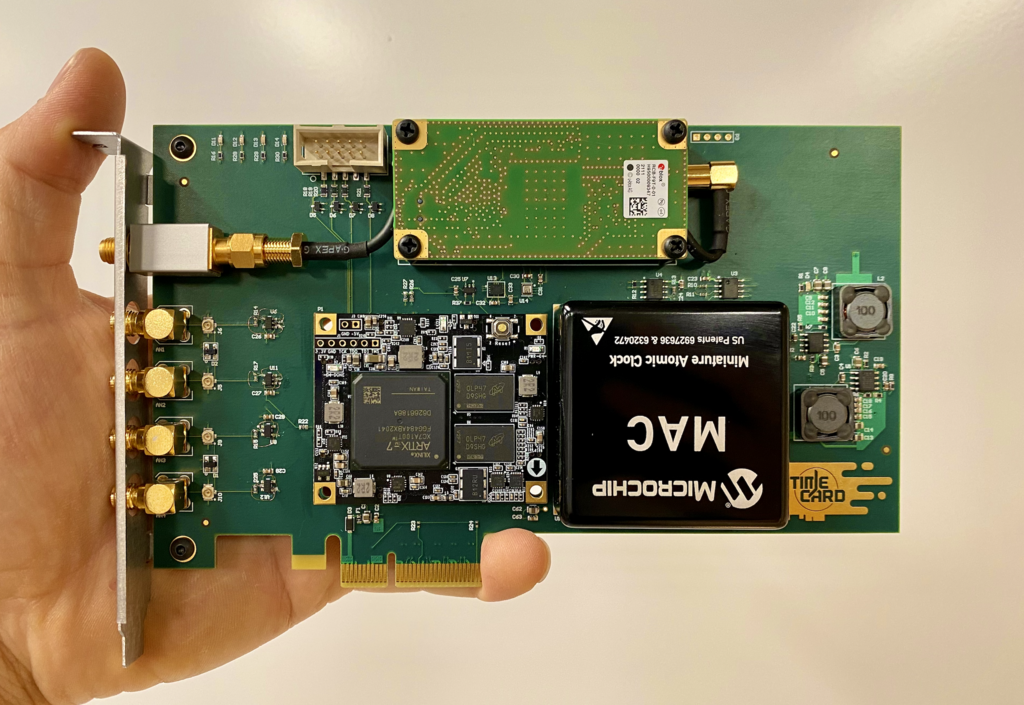
To manage the clock's output and steer a more stable, less expensive local oscillator (like a crystal oscillator), satellites use a critical piece of circuitry: a Phase-Locked Loop (PLL). The PLL constantly compares the local oscillator's phase against the atomic reference. It then generates a correction signal to adjust the local oscillator's frequency, effectively 'locking' it to the stability of the atomic clock while filtering out some of the short-term noise.

Let's review the key terms we've covered for establishing a local time scale.

Now, test your understanding of how satellite clocks are characterised.

This carefully characterised local time scale is the first step. It provides a stable, predictable foundation upon which the entire satellite constellation will be synchronised.