Probability Theory

The Building Blocks of Chance

At its heart, probability is the mathematics of uncertainty. It gives us a formal way to reason about things that are not guaranteed to happen. To do this, we need a solid foundation, which starts with the idea of a probability space.

A probability space has three key ingredients:

Sample Space (Ω): This is the set of all possible outcomes of an experiment. If you roll a standard six-sided die, the sample space is {1, 2, 3, 4, 5, 6}. If you flip a coin, it's {Heads, Tails}.
Events (F): An event is a specific outcome or a set of outcomes you're interested in. For the die roll, "rolling an even number" is an event, corresponding to the set {2, 4, 6}. "Rolling a 5" is also an event, corresponding to the set {5}.
Probability Measure (P): This is a rule that assigns a number between 0 and 1 to every event. A probability of 0 means the event is impossible, while a probability of 1 means it's certain. For a fair die, the probability of rolling any specific number is 1/6.

Together, these three parts give us a complete framework for describing a random process.

Turning Outcomes into Numbers

In data science, we need to perform calculations on the results of random processes. It’s hard to do math with outcomes like "Heads" or "Tails." We need a way to convert these outcomes into numbers. This is the job of a random variable.

Random Variable

noun

A variable whose value is a numerical outcome of a random phenomenon. It maps outcomes from the sample space to real numbers.

Let's imagine an experiment where we flip a coin twice. The sample space is {HH, HT, TH, TT}. We can define a random variable, let's call it $X$ , to be the total number of heads.

Outcome	Number of Heads (Value of X)
HH	2
HT	1
TH	1
TT	0

Now, instead of talking about abstract outcomes, we can analyze the numerical values of $X$ : 0, 1, and 2. This is much more useful for statistical analysis.

Describing Random Behavior

Once we have a random variable, we want to know how likely its different values are. This is described by its probability distribution, which tells us how the total probability of 1 is spread across all possible values.

For a discrete random variable (one that can only take specific values, like our coin flip example), this is called a Probability Mass Function (PMF). It gives the exact probability for each possible value.

For our double coin flip, the PMF of $X$ (number of heads) is: $P(X=0) = 1/4$ $P(X=1) = 2/4 = 1/2$ $P(X=2) = 1/4$

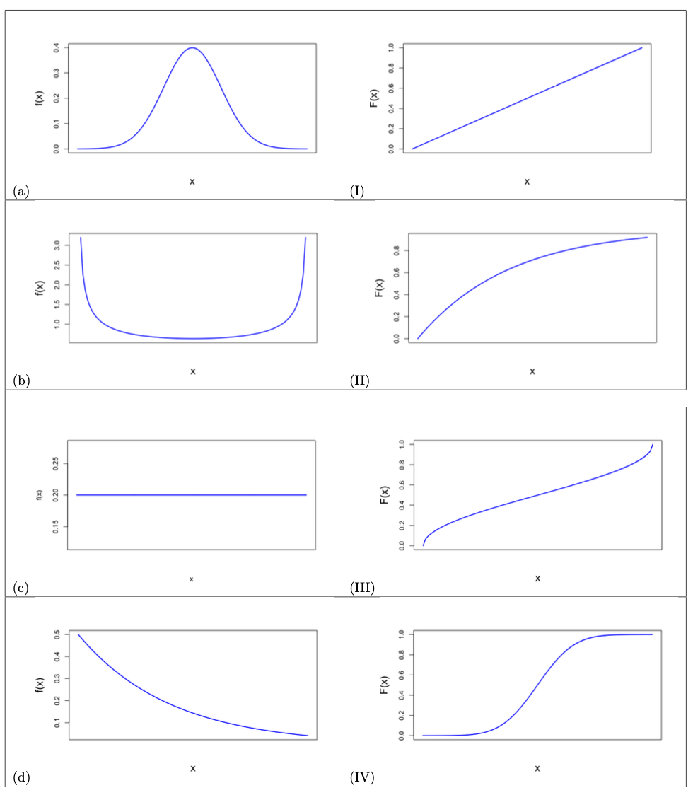
Notice that the probabilities sum to 1. For a continuous random variable (one that can take any value in a range, like a person's height), we use a Probability Density Function (PDF). The area under the curve of a PDF over a certain range gives the probability of the variable falling within that range.

Summarizing Distributions

A full probability distribution gives us complete information, but often we want to summarize it with just a couple of numbers. The two most important summaries are the expectation and the variance.

Expectation ( $E[X]$ ), or the expected value, is the long-run average value of a random variable. It's a weighted average of all possible values, where the weights are the probabilities.

E[X] = \sum_{i} x_i P(X=x_i)

For our double coin flip example, the expected number of heads is:

E[X] = (0 \times \frac{1}{4}) + (1 \times \frac{1}{2}) + (2 \times \frac{1}{4}) = 0 + \frac{1}{2} + \frac{1}{2} = 1

This makes sense: if you flip two coins many times, you'd expect to get one head on average.

Variance ( $Var(X)$ ) measures how spread out the values of a random variable are from its expected value. A low variance means the outcomes are tightly clustered around the average, while a high variance means they are more spread out.

Var(X) = E[(X - E[X])^2]

A more practical measure of spread is the standard deviation ( $\sigma$ ), which is simply the square root of the variance ( $\sigma = \sqrt{Var(X)}$ ). It's in the same units as the random variable, making it easier to interpret.

From Theory to Reality

So far, we've talked about theoretical probabilities. But how do we know they reflect what happens in the real world? This is where one of the most important ideas in all of probability comes in: the Law of Large Numbers.

The theoretical underpinnings particularly justified by statistical inference methods are together termed as statistical learning theory.

The Law of Large Numbers states that as you repeat an experiment a large number of times, the average of the results will get closer and closer to the expected value.

If you flip a fair coin 10 times, you might get 7 heads (an average of 0.7). But if you flip it 10,000 times, the average number of heads will be extremely close to the expected value of 0.5. This principle is what makes casinos profitable and insurance companies stable. It's the bridge that connects theoretical probability to the frequencies we observe in real data.

Ready to test your understanding of these core concepts?

Quiz Questions 1/6

What are the three essential components of a probability space?

Quiz Questions 2/6

If you roll two standard six-sided dice, what is the size of the sample space (i.e., the total number of possible outcomes)?

These foundational ideas are the bedrock of data science. They allow us to model the uncertainty inherent in data and build tools that make predictions in a world that is fundamentally random.

Applied Statistics for Data Science