You already know that raw data is rarely ready for a machine learning model. Cleaning missing values and converting categories with one-hot encoding are essential first steps. But to unlock a model's true potential, we need to go further and mathematically sculpt our features.

This isn't just about cleaning; it's about reshaping the data to better reveal the patterns hidden within. Let's start with scaling, a crucial step for a specific family of algorithms.

Consider a dataset for predicting house prices with two features: square footage (e.g., 1000-3000) and number of bedrooms (e.g., 2-5). The scale is vastly different. For models that use gradient descent to find the optimal solution, this is a problem.

Imagine a valley where the lowest point is the best model solution. If the scales are unequal, the valley is stretched into a long, narrow ellipse. The gradient descent algorithm will zig-zag inefficiently down the steep sides instead of taking a direct path to the bottom. Scaling transforms this valley into a more circular shape, allowing the algorithm to find the minimum much faster.

Common scaling methods like Standardization (Z-score normalisation) or Min-Max scaling ensure all features have a similar range, which is critical for algorithms like linear regression, logistic regression, and neural networks. However, tree-based models like Decision Trees and Random Forests are largely immune to feature scaling because they split data one feature at a time, irrespective of the other features' ranges.

Categorical features with thousands of unique values, known as high-cardinality features, pose a serious challenge. A 'Postcode' column, for instance, could create thousands of new columns if you used one-hot encoding, making your dataset unwieldy and potentially harming model performance.

A more sophisticated technique is Target Encoding. Instead of creating binary flags, it replaces each category with the average value of the target variable for that category. For example, to predict delivery time, you could replace each postcode with the average delivery time for all orders going to that postcode.

This is powerful but carries a risk of data leakage. You're using information from the target variable to create a feature. To mitigate this, practitioners often use techniques like adding smoothing or calculating the means on folds of the data not being trained on.

Another common issue is skewed data distributions. Features like income or website visits often have a long tail, where most values are clustered at the low end and a few are extremely high. This can violate the assumptions of linear models and disproportionately influence the model's learning process.

A simple fix is the logarithmic transformation, which compresses the range of the long tail.

For more flexibility, the Box-Cox transformation can find the best power transformation to stabilise variance and make the data more normal-like. It uses a parameter, lambda ($\\lambda$), to find an optimal fit.

Sometimes the most predictive information isn't in the original features, but in their relationships. Polynomial feature generation creates new features by combining or transforming existing ones.

Imagine predicting house prices from 'width' and 'length' features. A simple linear model might struggle to capture their combined effect. By creating an interaction term ('width' * 'length'), we create a new feature for 'area', which is far more predictive.

We can also create polynomial features by raising a single feature to a power (e.g., $x^2$, $x^3$). This can help a linear model capture non-linear relationships in the data.

While creating features is powerful, it can also add noise. With dozens or hundreds of features, how do we select the most important ones? This is where automated feature selection comes in.

One method is to use Lasso Regression (L1 regularisation). It's a type of linear regression that penalises the model for having too many features. During training, it shrinks the coefficients of less important features towards zero. Any feature whose coefficient becomes exactly zero can be safely discarded.

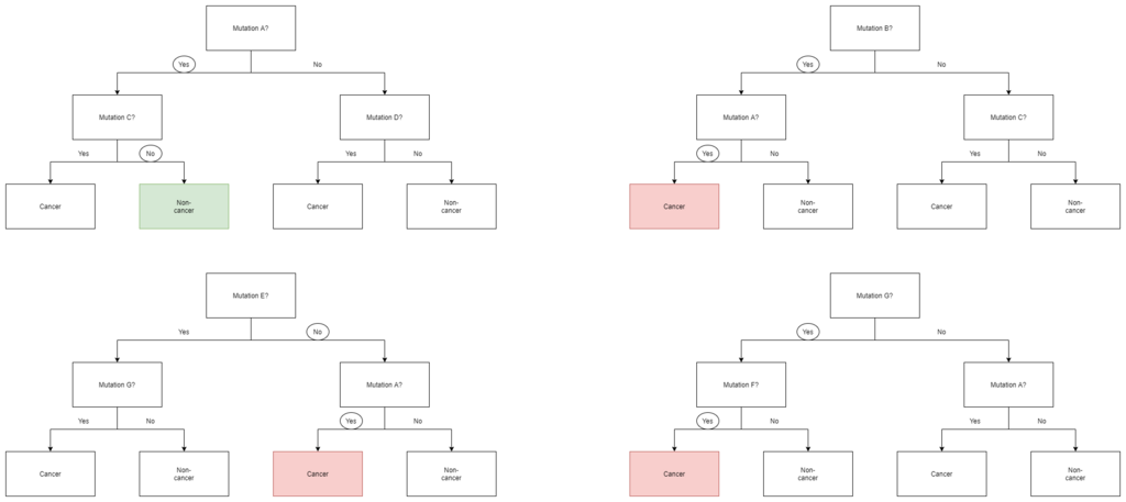
Another popular approach is using tree-based feature importance. Models like Random Forest and Gradient Boosting internally calculate how much each feature contributes to reducing impurity or error across all the decision trees in the ensemble. We can then rank the features by this score and select the top N, effectively filtering out the noise.

Feature engineering is an iterative process of creation, transformation, and selection. By mastering these advanced techniques, you can move beyond default settings and build models that are not only more accurate but also more robust and interpretable.

Time to test your understanding of these feature engineering techniques.