Applied Machine Learning Algorithms
Linear Regression Math
The Cost of Being Wrong
Every model makes predictions, but how do we know if those predictions are any good? We need a way to measure the model's error. In linear regression, the most common way to do this is with a cost function, specifically the Mean Squared Error (MSE). The goal is to find the line that makes this error as small as possible.
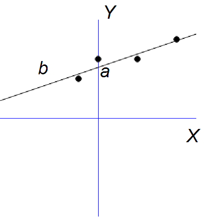
Imagine you have a set of data points. A linear model draws a straight line through them. The error for a single point is the vertical distance between the actual data point and the point predicted by the line. This distance is called a residual. To calculate the total error for the whole dataset, we can't just add up the residuals, because some will be positive and some negative, and they might cancel each other out. To solve this, we square each residual first. This makes all the error values positive. Finally, we take the average of all these squared residuals. That's the Mean Squared Error.
The entire process of training a linear regression model is about finding the specific values for the model's parameters, its slope and intercept, that result in the lowest possible MSE.
The Downhill Path with Gradient Descent
Minimizing the MSE is like standing on a hillside in a thick fog and trying to find the lowest point in the valley. You can't see the bottom, but you can feel which way is downhill from where you are. You take a step in that direction, check the slope again, and take another step. You repeat this until you can't go any further down. This is the core idea behind an iterative optimization algorithm used to find the minimum of a function.
In the context of linear regression, the 'hillside' is the cost function, and the 'location' is defined by the current values of our model's parameters (let's call them for the intercept and for the slope). The 'downhill direction' is given by the partial derivative of the cost function with respect to each parameter. We update the parameters by taking a small step in the negative direction of this gradient. The size of that step is controlled by a value called the learning rate, symbolized by (alpha).
A small learning rate means tiny, slow steps, but it's unlikely to overshoot the minimum. A large learning rate gets you there faster, but you risk overshooting the bottom and bouncing around, or even diverging completely. The process is repeated until the change in the cost function becomes negligible, meaning we've reached the bottom.
The Direct Route with the Normal Equation
Gradient descent is iterative, but what if there was a way to solve for the optimal parameters directly, in one mathematical step? There is, and it's called the It's an analytical approach that comes from the calculus of finding a minimum: you take the derivative of the cost function, set it to zero, and solve. When applied to the MSE cost function in matrix form, this derivation gives us a beautiful, compact formula.
So why use gradient descent if the Normal Equation can solve the problem in one shot? The trade-off is computational complexity. Calculating the inverse of a matrix, , is a very expensive operation. For a dataset with features, this is roughly an operation. If you have thousands of features, this becomes computationally infeasible.
Gradient descent, on the other hand, works well even with millions of features. The Normal Equation is great for smaller datasets where the number of features is in the hundreds or low thousands, but for the massive datasets common in modern machine learning, gradient descent is the go-to method.
Rules of the Road
Linear regression is powerful, but its results are only reliable if certain assumptions about the data hold true. Violating these assumptions can lead to misleading or completely incorrect conclusions.
| Assumption | What it Means | Why it Matters |
|---|---|---|
| Linearity | The relationship between the predictor variables and the target variable is linear. | If the true relationship is curved (e.g., quadratic), a straight line will be a poor fit, and the model's predictions will be systematically wrong. |
| Independence | The errors (residuals) are independent of each other. | If errors are correlated (e.g., in time-series data where one observation influences the next), our confidence in the model's accuracy will be artificially inflated. |
| Homoscedasticity | The errors have a constant variance at every level of the predictor variables. | If the variance of the error changes (heteroscedasticity), predictions will be more reliable for some ranges of the predictors than for others, making the model untrustworthy overall. |
| Normality of Errors | The errors are normally distributed. | This assumption is most critical for constructing reliable confidence intervals and conducting hypothesis tests about the model's parameters. |
Checking these assumptions, often through visual inspection of residual plots, is a crucial step in the modeling process. It ensures that the mathematical machinery of linear regression is being applied in a situation where it can actually succeed.
What is the primary purpose of the Mean Squared Error (MSE) in linear regression?
When calculating the Mean Squared Error (MSE), why are the individual errors (residuals) squared?