Applied Foundations of Credit Risk Modeling
PD Modeling Techniques
From Data to Default Probability
At its core, a credit risk model answers a simple question: What is the chance this borrower will fail to pay back their loan? To get that answer, we need to transform raw borrower data—income, credit history, loan amount—into a single, standardized number: the Probability of Default (PD).
For decades, the go-to tool for this job has been logistic regression. It’s a statistical method perfectly suited for binary outcomes. A borrower either defaults or they don't. There's no in-between. Logistic regression takes various input variables and maps them to a probability between 0 and 1.
The output isn't a simple linear prediction. Instead, the model calculates the log-odds of default. This value is then passed through the sigmoid function, which squishes any number into a neat 0-to-1 probability. The beauty of this approach is its transparency. Each coefficient () tells you exactly how much a single factor, like a $10,000 increase in annual income, influences the odds of default. This interpretability is why regulators have historically favored it.
Choosing the Right Ingredients
A model is only as good as the data it's fed. Before we can even think about building a PD model, we need to select and refine our input variables, or features.
This process, known as feature engineering and selection, is part art, part science. Feature engineering involves creating new, more insightful variables from existing ones. For instance, instead of using 'total debt' and 'annual income' as separate inputs, we could engineer a 'debt-to-income ratio'. This single feature often has more predictive power than its individual components.
Once we have a pool of potential features, we must select the best ones. Simply throwing every available piece of data into the model is a bad idea. It can lead to overfitting, where the model learns the noise in the training data instead of the underlying patterns. It also introduces issues like multicollinearity, where two or more variables are highly correlated, making it difficult to isolate their individual effects on the outcome. Analysts use statistical techniques like calculating Information Value (IV) or using automated stepwise selection to find a potent but stable set of predictors.
Good feature selection ensures the model is both predictive and robust, capturing real risk drivers without being overly complex or unstable.
The New School of Models
While logistic regression is a reliable workhorse, machine learning (ML) models like Random Forests and Gradient Boosting Machines (GBMs) have become powerful challengers. Instead of relying on a single, elegant equation, these models use an ensemble of decision trees to make predictions.
A random forest, for example, builds hundreds or even thousands of individual decision trees, with each tree getting a slightly different subset of the data. To make a prediction, the model tallies the 'votes' from all the trees. This approach allows the model to capture complex, non-linear relationships in the data that logistic regression might miss.
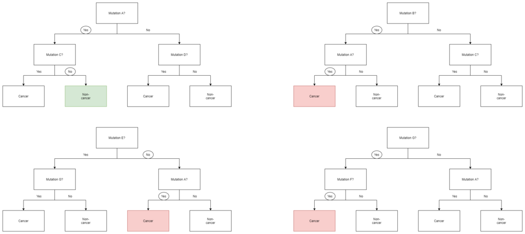
This leads to the central trade-off in modern credit modeling: predictive power versus interpretability. ML models often deliver higher accuracy—they are better at distinguishing between defaulters and non-defaulters. But they are also 'black boxes'. It's difficult to pinpoint exactly why a GBM denied a specific applicant. You can't easily point to a coefficient and explain its impact.
Logistic regression, on the other hand, is fully transparent. This makes it easier to explain decisions to customers and to satisfy regulators who require clear, auditable models. The choice between a traditional model and an ML model often depends on the institution's risk appetite, regulatory environment, and technical capabilities.
| Model Type | Primary Benefit | Primary Drawback |
|---|---|---|
| Logistic Regression | High Interpretability | May miss non-linear patterns |
| Random Forest / GBM | High Predictive Power | 'Black Box' nature |
| Neural Networks | Can model deep complexities | Requires vast data, hard to explain |
A Matter of Timing
Finally, a crucial aspect of PD modeling is the economic context. Models can be built to reflect risk at a specific moment or over an entire economic cycle.
A Point-in-Time (PIT) model estimates the probability of default based on the current economic conditions. If the economy is booming, a PIT model will produce lower PDs because default rates are generally low. If a recession hits, the model's PDs will rise sharply. These models are highly responsive but can be volatile.
A Through-the-Cycle (TTC) model aims to estimate an average PD over the course of a full economic cycle, smoothing out the peaks and troughs. It answers the question: what is the borrower's default risk under 'normal' economic conditions? TTC models are more stable, which is useful for long-term capital planning, but they are less responsive to immediate changes in the economic climate.
Many banks use a hybrid approach, starting with a TTC baseline and applying PIT adjustments to reflect the current reality. This gives them both a stable, long-term view and an accurate picture of near-term risk.
With these modeling techniques, banks can systematically evaluate risk and make informed lending decisions.
In a logistic regression model for credit risk, what is the primary role of the sigmoid function?
A credit risk analyst is building a model to estimate a borrower's default risk under 'normal' economic conditions, smoothing out the effects of short-term booms or recessions. Which type of model are they building?