Sequence Alignment Algorithms

The Blueprint of Comparison

Comparing two biological sequences isn't as simple as checking if they are identical. Evolution introduces changes: substitutions, insertions, and deletions. Sequence alignment algorithms are the computational tools we use to find the best possible pairing between two sequences, accounting for these changes. The goal is to infer homology—a shared ancestry—or functional similarity.

There are two primary philosophies for alignment: global and local.

A global alignment forces the alignment to span the entire length of both sequences. It’s like comparing two complete sentences to see how similar they are overall.

A local alignment, on the other hand, seeks out the regions of highest similarity within the sequences, ignoring the parts that don't match well. It’s like finding the same key phrase within two different books.

Feature	Global Alignment (Needleman-Wunsch)	Local Alignment (Smith-Waterman)
Goal	Align entire sequences from end to end.	Find the best matching subsequences.
Use Case	Comparing two closely related genes of similar length.	Finding conserved domains or motifs in proteins.
Output	A single alignment representing the full sequences.	One or more high-scoring local alignments.

Global Alignment with Needleman-Wunsch

The Needleman-Wunsch algorithm is a classic method that guarantees finding the optimal global alignment. It uses to build a solution incrementally. Imagine a grid where one sequence forms the top row and the other forms the first column. Each cell in this grid will store the score of the best possible alignment up to that point.

To fill any cell in the grid, you consider three possibilities:

Match/Mismatch: Align the corresponding characters from each sequence. The score is the value of the top-left diagonal cell plus the score for this specific match or mismatch.
Deletion: Align a character from the vertical sequence with a gap in the horizontal one. The score is the value of the cell directly above plus the gap penalty.
Insertion: Align a character from the horizontal sequence with a gap in the vertical one. The score is the value of the cell directly to the left plus the gap penalty.

You choose the path that gives the highest score. After filling the entire matrix, the score in the bottom-right cell is the score of the optimal global alignment. To reconstruct the alignment itself, you trace back from this cell to the origin, following the path of decisions that led to the highest scores.

Finding Hotspots with Smith-Waterman

The Smith-Waterman algorithm modifies Needleman-Wunsch to perform local alignment. This is often more useful in biology, as we might want to find a conserved functional domain (like a binding site) within two otherwise dissimilar proteins.

The algorithm introduces two crucial changes:

No Negative Scores: If the calculated score for a cell is negative, it's set to 0. This allows an alignment to restart from any point, effectively ignoring regions of poor similarity.
Traceback from the Max: The traceback doesn't start at the bottom-right corner. Instead, it begins at the cell with the highest value anywhere in the matrix and stops as soon as it reaches a cell with a score of 0.

This simple adjustment allows the algorithm to pinpoint the most similar subsequences, no matter where they are located.

# A simplified Smith-Waterman implementation

def smith_waterman(seq1, seq2, match=2, mismatch=-1, gap=-1):
    rows = len(seq1) + 1
    cols = len(seq2) + 1
    matrix = [[0 for _ in range(cols)] for _ in range(rows)]
    max_score = 0
    max_pos = (0, 0)

    # Fill the scoring matrix
    for i in range(1, rows):
        for j in range(1, cols):
            match_score = matrix[i-1][j-1] + (match if seq1[i-1] == seq2[j-1] else mismatch)
            delete_score = matrix[i-1][j] + gap
            insert_score = matrix[i][j-1] + gap
            
            # The key difference: scores can't be negative
            score = max(0, match_score, delete_score, insert_score)
            matrix[i][j] = score

            # Track the highest score
            if score > max_score:
                max_score = score
                max_pos = (i, j)

    # Traceback would start from max_pos
    # ... (traceback logic not shown for brevity)

    return max_score, max_pos, matrix

# Example usage
seq_a = "AGCACACA"
seq_b = "ACACACTA"
max_score, max_pos, matrix = smith_waterman(seq_a, seq_b)
print(f"Highest local alignment score: {max_score} at position {max_pos}")

Smarter Scoring

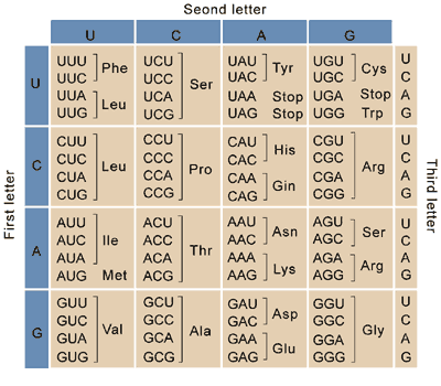
A simple match/mismatch score is a blunt instrument. In reality, some amino acid substitutions are more likely than others. For example, replacing one small, hydrophobic amino acid (like valine) with another (like isoleucine) is a common, conservative change. Replacing it with a large, charged amino acid (like arginine) is a drastic change that would likely disrupt protein function.

This is where substitution matrices come in. They are pre-calculated tables that assign a score for every possible amino acid substitution based on observed evolutionary frequencies.

Two families of matrices dominate bioinformatics:

PAM (Point Accepted Mutation): Derived from global alignments of closely related proteins. A PAM1 matrix corresponds to an evolutionary divergence of 1 accepted mutation per 100 amino acids. Higher PAM numbers (e.g., PAM250) are extrapolated for comparing more distant sequences.
(Blocks Substitution Matrix): Derived from local alignments of conserved sequence blocks (regions without gaps). A BLOSUM62 matrix, for example, is calculated from blocks with at least 62% sequence identity. Unlike PAM, higher BLOSUM numbers (e.g., BLOSUM80) are used for more closely related sequences, while lower numbers (BLOSUM45) are for more distant ones.

Another level of sophistication comes from gap penalties. A single large deletion event is more likely than a series of individual deletions. An models this by using two penalties: a high cost to open a gap (the first insertion/deletion) and a lower cost to extend it (for subsequent ones).

Speeding Things Up with BLAST

While Needleman-Wunsch and Smith-Waterman are thorough, they are too slow for searching massive databases with billions of base pairs. That's where heuristics come in. The Basic Local Alignment Search Tool (BLAST) is a family of programs that trades guaranteed optimality for immense speed.

BLAST doesn't compare every base. Instead, it follows a three-step process:

Seeding: It breaks your query sequence into short 'words' (e.g., 11 bases for DNA, 3 for proteins) and finds all the exact matches for these words in the database.
Extending: It then tries to extend these short, high-scoring 'seeds' in both directions, adding to the alignment score as long as it stays above a certain threshold.
Evaluating: Finally, it assesses the statistical significance of these extended hits. It calculates an Expect value (E-value), which represents the number of hits you would expect to see by chance. A lower E-value signifies a more significant, and likely biologically relevant, match.

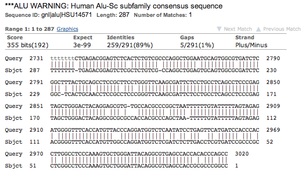
This seed-and-extend approach allows BLAST to quickly discard irrelevant sequences and focus its computational power only on promising candidates. It's a pragmatic solution that has become an indispensable tool in genomics, balancing the need for accuracy with the practical demands of big data.

Quiz Questions 1/6

What is the primary goal of performing a sequence alignment between two biological sequences?

Quiz Questions 2/6

Which statement best describes the fundamental difference between the Needleman-Wunsch and Smith-Waterman algorithms?

These algorithms form the computational foundation of modern bioinformatics, enabling us to decode the evolutionary and functional stories written in the language of DNA and proteins.

Applied Bioinformatics and Data Analysis