Algorithm Design and Analysis Fundamentals
Algorithm Analysis
Measuring Efficiency
Getting the right answer is only half the battle. A truly good algorithm gets the right answer efficiently. But how do we measure efficiency? We can't just time an algorithm with a stopwatch. The result would change depending on the computer's speed, the programming language, and other factors.
Instead, we analyze algorithms by looking at how their resource needs change as the size of the input grows. The two main resources we care about are time and space.
- Time Complexity: How many steps does an algorithm take to complete, relative to the input size?
- Space Complexity: How much memory does an algorithm need, relative to the input size?
Think of it like following a recipe. A simple recipe might say "mix all ingredients in one bowl." The space complexity is low (one bowl). A complex recipe might require multiple bowls for different stages, increasing its space complexity. Similarly, the time it takes depends on the number of steps. We want a way to describe these requirements that is independent of the specific kitchen or chef.
The Language of Growth
To talk about complexity, we use a special language called Big O notation. It's a way to describe the upper bound of an algorithm's running time or space usage. Essentially, Big O tells us how the number of operations grows as the input size () gets very large.
It focuses on the big picture. We're not interested in the exact number of steps, but in the overall growth rate. Big O notation simplifies things by ignoring constants and lower-order terms. For example, an algorithm that takes steps is simplified to just , because as becomes huge, the term dominates everything else.
Let's look at some common Big O classifications.
— Constant Time The algorithm takes the same amount of time regardless of the input size. Accessing the first item in a list is a classic example. Whether the list has 10 items or 10 million, getting the first one takes just one step.
— Linear Time The number of operations grows in a straight line with the input size. If you double the input, you roughly double the time. Reading every item in a list once, like in a linear search, is .
— Logarithmic Time This is incredibly efficient. The number of operations grows very slowly as the input size increases. Each time you double the size of the input, you only add one extra step. Binary search, which we'll discuss soon, is a prime example.
— Quadratic Time The number of operations grows with the square of the input size. If you double the input, the work roughly quadruples. A simple example is an algorithm that compares every item in a list to every other item.
Best, Worst, and Average
An algorithm's performance isn't always the same for inputs of the same size. It can depend on the arrangement of the data. This gives us three scenarios to consider: the best case, the worst case, and the average case.
Let's use linear search as our example. The goal is to find a specific number in an unordered list by checking each element one by one.
- Best Case: The number you're looking for is the very first element. You find it on your first try. The time complexity is because it takes a single step, no matter how long the list is.
- Worst Case: The number is the very last element, or it's not in the list at all. You have to check every single element to be sure. The time complexity is .
- Average Case: On average, you'd expect to find the item somewhere in the middle of the list. This would take roughly steps. In Big O notation, we drop the constant (), so the average case is also .
When we talk about the Big O of an algorithm, we are usually referring to its worst-case performance. It provides a guarantee: the algorithm will perform at least this well, and will never be slower.
Analyzing Recursive Algorithms
Analyzing loops is fairly straightforward, but what about algorithms that call themselves? This is recursion. To analyze a recursive algorithm, we use something called a recurrence relation.
A recurrence relation is an equation that defines a function in terms of its own previous values. It has two parts: the work done inside the function itself, and the work done by the recursive calls.
Let's apply this to binary search. This algorithm finds an item in a sorted list by repeatedly dividing the search interval in half. It checks the middle element. If it's a match, we're done. If the target is smaller, we repeat the search on the left half. If it's larger, we search the right half.
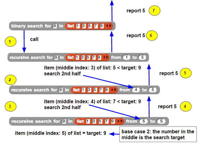
How does this look as a recurrence relation? In each step, binary search makes just one recursive call () on a problem that is half the size (). The work done in each step is constant—just a single comparison—so .
This gives us the relation: .
When you solve this relation (using methods beyond the scope of this introduction, like the Master Theorem), you find that the complexity is . This confirms our earlier statement: binary search is extremely fast because it cuts the problem in half with every step.
| Algorithm | Best Case | Average Case | Worst Case |
|---|---|---|---|
| Linear Search | |||
| Binary Search |
Understanding how to analyze an algorithm's efficiency is a fundamental skill. It allows you to make informed decisions and choose the right tool for the job, ensuring your programs are not just correct, but also scalable and performant.