Advancing through the AI Landscape
Neural Optimization Mechanics
The Engine of Learning
Training a neural network is an optimization problem. We have a loss function that tells us how wrong the network's predictions are, and our goal is to adjust the network's weights and biases to make that loss as small as possible. The core mechanism for this is backpropagation.
Imagine the loss function as a vast, hilly landscape. Our goal is to find the lowest valley. Backpropagation is like a compass that tells us which way is downhill from our current position. It works by calculating the gradient of the loss function with respect to each weight in the network. This gradient is just a vector that points in the direction of the steepest ascent. To descend, we simply take a step in the opposite direction.
To calculate these gradients, especially in deep networks with many layers, backpropagation relies on the chain rule from calculus. The chain rule allows us to compute the derivative of a composite function. Since a neural network is essentially a massive nested function (each layer's output is the next layer's input), the chain rule is the perfect tool. It lets us calculate the error contribution of each weight, layer by layer, starting from the output and working backwards to the input.
This process efficiently computes the gradients for all weights, telling us exactly how to adjust them to improve the model's performance.
Gradient Descent in Practice
Once we have the gradients, we use an algorithm called gradient descent to update the weights. The simplest version, often called Batch Gradient Descent, calculates the gradient using the entire training dataset before taking a single step. This is accurate but computationally expensive and impractical for large datasets.
In practice, we use variations that are much more efficient. The two most common are Stochastic Gradient Descent (SGD) and Mini-batch Gradient Descent.
| Method | Gradient Calculation | Update Frequency | Pros & Cons |
|---|---|---|---|
| Stochastic (SGD) | Uses a single training example. | After every example. | Pros: Fast updates. Cons: Very noisy; path to minimum is erratic. |
| Mini-batch | Uses a small batch of examples (e.g., 32, 64). | After every batch. | Pros: A good balance. Less noisy than SGD, more efficient than batch. Cons: Requires tuning the batch size. |
Mini-batch gradient descent is the standard for training deep learning models. It provides a stable compromise between the accuracy of using the full dataset and the speed of using a single example. The
Smarter Optimizers
Vanilla SGD can be slow. If the loss landscape is like a long, narrow ravine, SGD will oscillate back and forth across the steep sides instead of moving smoothly down the gentle slope of the ravine floor. To fix this, we use more advanced optimizers.
Momentum helps accelerate SGD in the correct direction. It adds a fraction of the previous update vector to the current one. This is like a heavy ball rolling downhill. It builds up momentum, smoothing out the oscillations and speeding up convergence, especially in ravines.
RMSProp (Root Mean Square Propagation) and Adam (Adaptive Moment Estimation) are adaptive optimizers. They maintain a separate learning rate for each parameter and adjust it during training. They give larger updates for infrequent parameters and smaller updates for frequent ones. Adam essentially combines the ideas of Momentum and RMSProp. It keeps track of both the momentum (first moment) and the variance of the gradients (second moment).
Adaptive optimizers like Adam often converge faster and require less manual tuning of the learning rate, making them a common default choice for many deep learning tasks.
Common Training Hurdles
Training deep networks isn't always smooth. Two notorious problems are the vanishing and exploding gradient problems.
As backpropagation moves from the output layer to the input layer, it multiplies gradients together. If these gradients are consistently small (less than 1), their product shrinks exponentially until it
The vanishing gradient problem occurs when the gradients used to update the weights during backpropagation diminish exponentially as they propagate through deep layers of a neural network.
This means the weights of the initial layers barely update, and the network fails to learn. Conversely, if gradients are consistently large (greater than 1), their product can explode, leading to massive weight updates that make the model unstable.
Several techniques were developed to combat these issues.
Weight Initialisation: Instead of initialising weights to zero or small random numbers, we use smarter schemes like Xavier or He initialisation. These methods set the initial weights based on the number of input and output neurons, ensuring gradients are in a reasonable range from the start.
Batch Normalisation: This technique normalises the output of a previous activation layer by subtracting the batch mean and dividing by the batch standard deviation. It's like resetting the distribution for each layer's input. This keeps the gradients flowing and allows for higher learning rates, which speeds up training. It's typically applied just before the activation function of a layer.
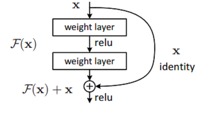
Residual Connections: In very deep networks, like ResNets, we can add
These create a shortcut for the gradient to flow through, bypassing several layers. This ensures that even in a network with hundreds of layers, the gradient can propagate back to the early layers without vanishing.
What is the primary purpose of the backpropagation algorithm in training a neural network?
Which variant of gradient descent offers a compromise between the computational efficiency of Stochastic Gradient Descent (SGD) and the stable convergence of Batch Gradient Descent?
These optimization mechanics are the foundation upon which modern deep learning models are built, enabling them to learn complex patterns from vast amounts of data.