An artificial neural network organises simple processing units, called neurons, into layers. The most common structure is the Multilayer Perceptron (MLP), which consists of an input layer, one or more hidden layers, and an output layer. The input layer receives the initial data, like the pixels of an image or the words in a sentence. The output layer produces the final result, such as a classification or a prediction.

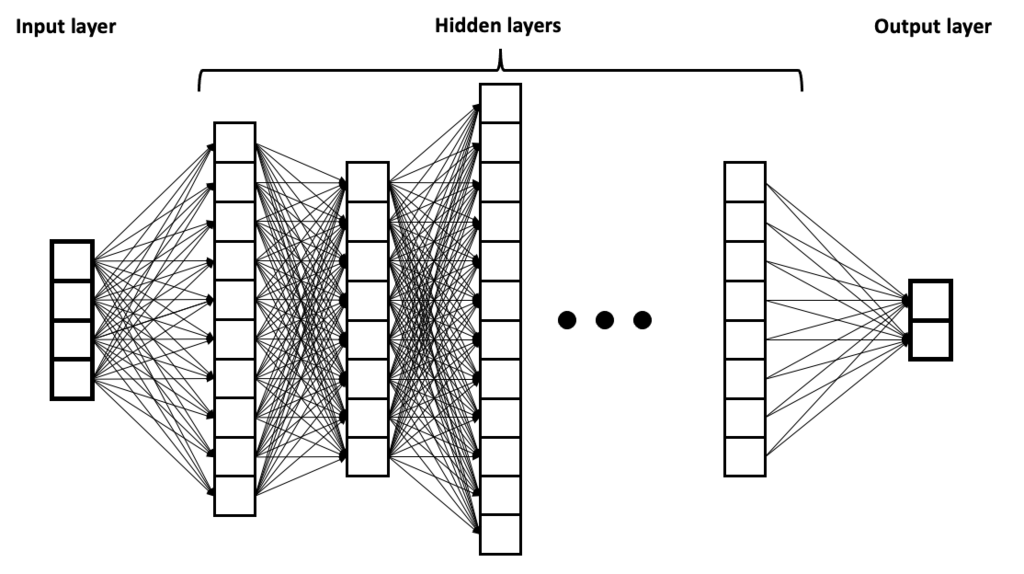
Between the input and output lie the hidden layers. This is where the network performs most of its computation, learning to recognise increasingly complex features from the data. Each neuron in a layer is connected to the neurons in the next, and information flows forward through the network. This process is called forward propagation.

Each connection has an associated weight, which determines the strength of the signal passed between neurons. A neuron sums up all the weighted inputs it receives, adds a bias, and then passes the result through an activation function to produce its output.

The activation function is a critical component. Without it, a neural network, no matter how many layers it has, would just be a linear function. It's the non-linearity introduced by activation functions that allows the network to learn complex relationships in the data.

Two common choices are the Sigmoid function and the Rectified Linear Unit (ReLU).

• Sigmoid: This function squashes its input into a range between 0 and 1. It was popular in early networks, but it has a major drawback. Its gradient is very small for large positive or negative inputs, which can slow down or even stop the learning process. This is known as the vanishing gradient problem.

• ReLU: This function is much simpler. It outputs the input directly if it's positive, and zero otherwise. It's computationally efficient and avoids the vanishing gradient problem for positive inputs, making it the most popular activation function for hidden layers today.

Before training begins, the network's weights must be set to some initial values. This isn't a trivial step. If all weights are initialised to zero, every neuron in a layer will compute the same output, making the network symmetrical and preventing it from learning. If they're set too large, the activation functions can saturate, leading to vanishing gradients. Weight initialisation strategies like Xavier or He initialisation are designed to set the initial weights in a way that avoids these problems, ensuring signals can flow effectively through the network.

A network learns by adjusting its weights to minimise the difference between its predictions and the actual target values. This process relies on two key mechanisms: a loss function and backpropagation.

A loss function measures how wrong the network's predictions are. For regression tasks, a common choice is Mean Squared Error (MSE), which penalises larger errors more heavily. For classification, Cross-Entropy Loss is often used because it's well-suited for measuring the difference between two probability distributions.

Once the loss is calculated, the network needs to figure out how to adjust each weight to reduce it. This is the job of backpropagation an algorithm that uses the chain rule from calculus to calculate the gradient of the loss function with respect to each weight in the network, starting from the output layer and working backwards.

This process, called gradient descent, is like walking down a hill blindfolded. The gradient tells you which way is steepest, and the learning rate determines the size of your step. The goal is to take steps downhill until you reach the bottom of the valley, which represents the minimum possible loss.

By repeatedly feeding data through the network (forward propagation), calculating the error, and adjusting the weights (backpropagation), the model gradually learns to make more accurate predictions.

Now, let's test your understanding of how these components fit together.

Understanding these architectural and mechanical details is the bridge from knowing what a neural network is to understanding how it actually works and learns from data.