Advanced Waves and Modern Electromagnetics
Wave Equation Derivation
From Fields to Waves
Maxwell's equations beautifully describe how electric and magnetic fields behave. They show a deep, codependent relationship: a changing magnetic field creates an electric field, and a changing electric field creates a magnetic field. But how do these interactions give rise to a self-propagating wave, like light?
To answer this, we need to manipulate the equations to describe one field in terms of itself. We'll combine the four first-order differential equations into a single, powerful second-order equation. This process reveals the wave hiding within the static laws.
First, we simplify our environment. We'll consider a source-free region of space, meaning there are no free charges () or currents (). This is like looking at the vacuum of space, far from any stars or planets. In this linear, isotropic, and homogeneous medium, Maxwell's equations become:
The Curl of the Curl
Our goal is to isolate the electric field, . We can start by taking the curl of Faraday's Law:
On the right side, we can swap the order of the curl and the time derivative, since they operate on different variables (space and time, respectively). This gives us:
Now, we can substitute Ampère-Maxwell's Law, , into the right side:
The left side, , can be simplified using a standard vector identity from calculus:
Applying this to our electric field , we get . Since we are in a source-free region, Gauss's Law tells us that . The first term vanishes, leaving us with just .
The Wave Equation Emerges
Now we equate our simplified left and right sides:
Cleaning this up, we arrive at the electromagnetic wave equation for the electric field, also known as the Helmholtz equation:
We can perform the exact same derivation for the magnetic field, , by starting with the curl of Ampère-Maxwell's Law and substituting Faraday's Law. The result is identical in form:
This is a profound result. The interconnectedness of electric and magnetic fields naturally gives rise to a wave that travels through space.
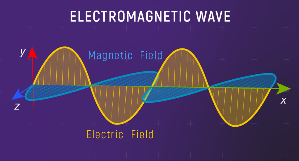
The general form of a one-dimensional wave equation is , where is the wave's speed. Comparing this to our derived equation, we can see that the speed of our electromagnetic wave is:
When Maxwell plugged in the known values for the () and the (), he calculated a speed of approximately meters per second. This was the known speed of light.
From this mathematical formulation, Maxwell determined that the speed of propagation of electromagnetic (EM) waves was the same as the speed of light, and thus showed that EM waves and visible light were really the same thing.
The Physics in the Math
The wave equation isn't just a mathematical abstraction. Its two key components have direct physical meaning.
The second-order time derivative, , represents the acceleration of the electric field at a point. It's not about how fast the field is changing, but how fast that change is changing. This acceleration is the engine of the wave, driving the oscillation forward.
The Laplacian operator, , describes the curvature or '-kinkiness-' of the field in space. It measures how much the value of the field at a point differs from the average value of its neighbors. A high Laplacian means the field is sharply curved, like at the peak or trough of a wave.
Laplacian
noun
The Laplacian operator, denoted as , is a differential operator that measures the difference between the value of a function at a point and the average value in its immediate neighborhood. In physical terms, it often relates to the flux density or curvature of a field.
The wave equation states that the acceleration of the field in time is proportional to its curvature in space. This is the essence of a self-propagating wave. Where the field is most curved (like the peak of a sine wave), it experiences the greatest acceleration, causing it to snap back and overshoot, creating the next part of the wave. This beautiful interplay allows the wave to travel through a vacuum, needing no medium, powered only by its own changing fields.
Let's check your understanding of this derivation.
What is the first key assumption made to simplify Maxwell's equations for the derivation of the electromagnetic wave equation?
The derivation of the wave equation for the electric field, , starts by taking the curl of which of Maxwell's equations?
By following a few logical steps of vector calculus, we've transformed Maxwell's static-looking rules into a dynamic equation that describes one of the universe's most fundamental phenomena: light.