Performance Analysis

Beyond Syntax: Measuring Efficiency

Writing code that works is one thing. Writing code that works efficiently is another. When you're dealing with a handful of items, almost any approach feels fast. But what happens when your list grows to a million entries, or a billion? Suddenly, small differences in how you structure your data can mean the difference between an app that runs instantly and one that grinds to a halt.

This is where performance analysis comes in. We need a consistent way to talk about how an algorithm's performance changes as the size of its input grows. Instead of relying on gut feelings or timing code on one specific machine, we use a formal system called Big O notation.

Big O notation is a powerful tool used in computer science to describe the time complexity or space complexity of algorithms.

Big O describes the upper bound, or worst-case scenario. It answers the question: as my data gets infinitely large, how does the number of operations scale? Let's say we have an input of size $n$ . If an algorithm has a complexity of $O(n)$ , we say it has linear time complexity. This means the number of operations grows in direct proportion to the size of the input. Double the data, and you roughly double the work.

If another algorithm has a complexity of $O(1)$ , it has constant time complexity. No matter how large the input is, the number of operations stays the same. Finding an item in a Python dictionary by its key is a classic example of an $O(1)$ operation.

Algorithm

noun

A finite sequence of well-defined, computer-implementable instructions, typically to solve a class of specific problems or to perform a computation.

Here are some of the most common Big O classifications you'll encounter, ordered from most to least efficient.

Notation	Name	Example
$O(1)$	Constant	Looking up an element in a dictionary by key.
$O(\log n)$	Logarithmic	Finding an item in a sorted array (binary search).
$O(n)$	Linear	Iterating through all elements in a list.
$O(n \log n)$	Log-Linear	Efficient sorting algorithms like Timsort (Python's default).
$O(n^2)$	Quadratic	Comparing every element to every other element (nested loops).
$O(2^n)$	Exponential	Solving the Traveling Salesperson problem with a brute-force approach.

Time vs. Space

When we analyze performance, we're usually balancing two key resources: time and memory.

Time complexity measures how many computational steps are needed. It's about the CPU cycles. When people mention Big O without specifying, they're almost always talking about time complexity.

Space complexity measures how much memory an algorithm needs to run. This includes the space for the input data plus any additional memory the algorithm allocates. Sometimes, you can make an algorithm faster by using more memory, a classic trade-off known as a time-space tradeoff.

For example, you could create a lookup table (using more space) to pre-calculate results, which would make future lookups much faster (saving time).

In modern computing, memory is often more plentiful than a user's patience, so time complexity is frequently prioritized. However, in memory-constrained environments like mobile devices or embedded systems, space complexity can be just as critical. Understanding both helps you make informed decisions about which data structure is right for the job.

Python Under the Hood

To truly grasp why Python's data structures perform the way they do, we need to peek at their underlying implementation in This is the original, and most widely used, implementation of Python, written in C.

Python lists, for instance, are not simple linked lists. They are implemented as dynamic arrays. This means they are a contiguous block of memory that can resize itself as needed. Getting an item by its index, my_list[i], is an $O(1)$ operation because the computer can calculate the memory address directly. However, inserting an item at the beginning of the list requires shifting every other element over, making it an $O(n)$ operation.

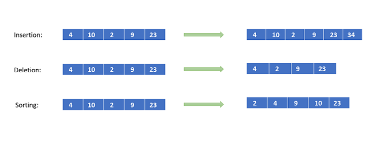
But what about appending? Adding an element to the end of a list is usually fast. Most of the time, it's an $O(1)$ operation because CPython allocates extra space at the end of the list to accommodate future appends. But what if that extra space runs out? The array must be resized. This involves allocating a new, larger block of memory and copying all the old elements over.

This copy is an expensive $O(n)$ operation. But since it happens only occasionally, we can say that appending has an amortized worst-case of $O(1)$ . Over a long sequence of appends, the cost of the occasional resize is spread out, and the average cost per append remains constant. This is a key concept called

Putting It to the Test

Theoretical analysis with Big O is essential, but sometimes you need to measure real-world performance. Python's built-in timeit module is the standard tool for this. It lets you run a small snippet of code millions of times to get an accurate measurement of its execution time, while avoiding common pitfalls of manual timing.

For example, let's compare the time it takes to check for membership in a list versus a set. A list requires scanning through elements one by one ( $O(n)$ ), while a set uses a hash table, just like a dictionary, for an average lookup time of $O(1)$ .

import timeit

# Setup strings for the tests
SETUP = """
import random
data = [random.randint(0, 10000) for _ in range(1000)]
search_val = data[500] # An element we know is in the middle
data_set = set(data)
"""

# Test membership in a list
list_test = timeit.timeit(stmt='search_val in data', setup=SETUP, number=10000)

# Test membership in a set
set_test = timeit.timeit(stmt='search_val in data_set', setup=SETUP, number=10000)

print(f"List search took: {list_test:.6f} seconds")
print(f"Set search took:  {set_test:.6f} seconds")

Running this code will show a dramatic difference. The set lookup will be orders of magnitude faster than the list lookup, clearly demonstrating the real-world impact of choosing the right data structure.

Time for a quick check on these concepts.

Let's test your understanding of performance analysis.

Quiz Questions 1/6

What does Big O notation primarily describe in the context of algorithm analysis?

Quiz Questions 2/6

Which of the following Big O notations represents the most efficient (fastest) time complexity for a large input size 'n'?

Understanding how to analyze performance is the first step toward writing truly professional code. It allows you to anticipate bottlenecks, choose the right tools, and build systems that scale gracefully.

Advanced Python Data Structures and Optimization