Advanced Probability Distributions
Advanced Probability Distributions
Beyond the Basics
You're likely familiar with basic probability and distributions like the Normal or Binomial. Now, we move past calculating simple odds and into the mathematical structure that defines random phenomena. A probability distribution isn't just a graph; it's a function that links every possible outcome of an experiment to its probability of occurring.
For any random variable , its distribution tells us everything we need to know about it. We'll be looking at this from a more rigorous, calculus-based perspective to understand the properties that make these distributions so useful.
Continuous Distributions
When a variable can take any value within a range, like height or temperature, we use a continuous distribution. The core concept here is the Probability Density Function, or PDF, denoted as . A key point to remember is that for a continuous variable, the probability of it taking on any single, exact value is zero. Think about it: what are the odds of a person being exactly 180.000... cm tall? Infinitesimally small.
Instead, we calculate the probability that a value falls within an interval by integrating the PDF over that interval. The probability that falls between and is:
Two of the most important properties of any distribution are its expected value and variance. For a continuous distribution, these are also found using integrals.
Beyond the Normal distribution, distributions like the Exponential distribution model the time between events in a Poisson process (e.g., time between customer arrivals), while the Gamma distribution can model the time until the -th event occurs.
Discrete Distributions
For variables that can only take specific, separate values, like the number of heads in five coin flips, we use discrete distributions. Here, we use a Probability Mass Function (PMF), denoted as , which gives the probability that the random variable is exactly equal to some value .
Unlike with continuous variables, for discrete variables, can be a non-zero value.
Calculating the expected value and variance for discrete distributions involves summations instead of integrals.
Beyond the Binomial distribution, the Poisson distribution is excellent for modeling the number of events occurring in a fixed interval of time or space (e.g., number of emails received per hour). The Geometric distribution models the number of trials needed to get the first success.
Working with Multiple Variables
Real-world problems rarely involve just one random variable. More often, we need to understand the relationship between two or more. This is where multivariate distributions come in. The simplest case is the bivariate distribution, which involves two variables, and .
The joint probability distribution gives the probability of and taking on specific values simultaneously. For discrete variables, this is written as . The sum of all possible joint probabilities must equal 1.
| Y = 0 | Y = 1 | Marginal P(X) | |
|---|---|---|---|
| X = 0 | 0.1 | 0.4 | 0.5 |
| X = 1 | 0.2 | 0.3 | 0.5 |
| Marginal P(Y) | 0.3 | 0.7 | 1.0 |
From the joint distribution, we can derive marginal distributions, which give the probability distribution of a single variable by itself. This is done by summing (for discrete) or integrating (for continuous) over the other variables. In the table above, the marginal probabilities are the sums of each row and column.
We can also find the conditional distribution, which describes the probability of one variable given that another has a certain value, like . This is fundamental to many statistical and machine learning models, as it allows us to update our beliefs about one variable based on information about another.
Applications in Machine Learning
Probability distributions are not just theoretical constructs; they are the engine of modern machine learning. In machine learning, we often want to build a model that can predict an outcome () based on some input features (). This is inherently a probabilistic task.
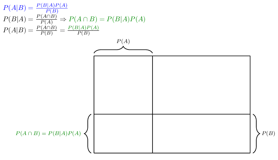
For example, in a classification problem (like identifying spam email), we can use Bayes' theorem to calculate the probability that an email is spam given its content. This requires modeling the distribution of words in spam versus non-spam emails. Logistic regression, a foundational classification algorithm, directly models the probability of a binary outcome.
In more advanced models, like generative models, the goal is to learn the entire probability distribution of the data itself. A model that learns the joint distribution of pixels in images of faces, for instance, can then be used to generate brand new, realistic-looking faces. Understanding the mathematical properties of distributions is crucial for designing, training, and troubleshooting these complex systems.
Let's test your understanding of these advanced concepts.
For a continuous random variable X described by a Probability Density Function (PDF), what is the probability of X taking on any single, exact value, such as ?
If you have the joint probability distribution of two random variables, X and Y, how do you find the marginal distribution of X?