You already know that price elasticity measures how much the quantity demanded of a good responds to a change in its price. But calculating elasticity as a simple percentage change between two points only gives you an average over that range. What if you need to know the elasticity at a single, specific point on the demand curve? This is crucial for making precise pricing decisions where even small adjustments matter.

For this, we need a more powerful tool. Instead of looking at the change between two points, we use calculus to find the instantaneous rate of change at one point. This method is called point elasticity.

To zoom in on a single point, we replace the Δ (delta), which represents a sizable change, with the derivative. The derivative dQ/dP gives us the exact slope of the demand curve at a specific point (P, Q).

A common misconception is that elasticity is constant along a demand curve. This is only true for a few special cases. For a typical linear demand curve, elasticity is different at every single point.

As the diagram shows, on a linear demand curve, elasticity is not the same as the slope. The slope is constant, but the P/Q ratio changes. At high prices and low quantities (top-left of the curve), demand is elastic. A price change causes a large percentage change in quantity. At the midpoint, demand is unit elastic. At low prices and high quantities (bottom-right), demand is inelastic, as the same price change now represents a much smaller percentage shift in the large quantity demanded.

While point elasticity is precise, sometimes you only have data for two separate points and need to find the arc elasticity between them. Using the standard percentage change formula can be misleading because the result depends on whether you calculate the change from point A to B or from B to A. The Midpoint Method solves this problem by using the average of the initial and final values for both price and quantity.

Let's say the price of a coffee drops from $3 to $2.50, and the quantity sold per day increases from 100 to 150 cups.

Using the midpoint method:

• Percentage change in quantity = (150 - 100) / ((100 + 150) / 2) = 50 / 125 = 40%
• Percentage change in price = (2.50 - 3.00) / ((3.00 + 2.50) / 2) = -0.50 / 2.75 = -18.2%

Elasticity = 40% / -18.2% ≈ -2.2. Since the absolute value (2.2) is greater than 1, demand is elastic in this price range.

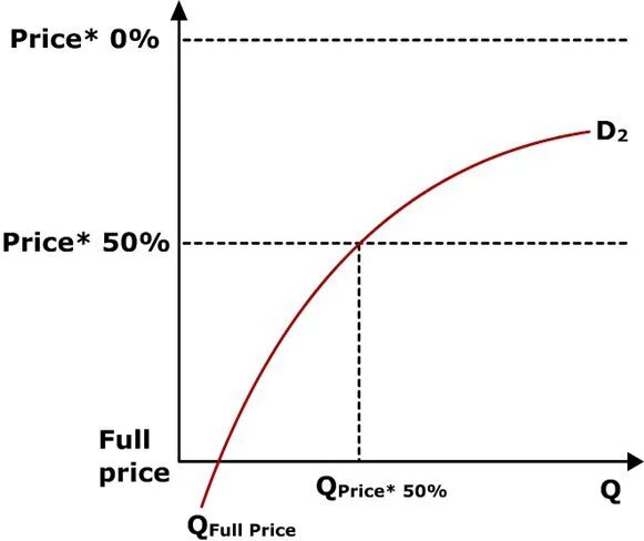
This method is especially useful for dealing with non-linear demand curves, where the slope is continuously changing. It provides a more accurate measure of elasticity over a range than the simple percentage change formula.

Understanding these more advanced methods allows for a much finer-grained analysis of market behavior, enabling better forecasting and more strategic pricing.

Let's test your understanding of these advanced elasticity calculations.

By moving beyond simple averages and using tools like derivatives and the midpoint formula, you can analyze demand with much greater precision.