Ohm's Law and Kirchhoff's Laws are the bedrock of circuit analysis. For simple circuits, you can often find what you need by reducing series and parallel resistors. But as circuits get more complex, with multiple sources and interconnected loops, this approach breaks down. It becomes a puzzle with no clear starting point.

To tackle this complexity, we need systematic methods. Nodal and Mesh analysis are two powerful techniques that provide a clear, step-by-step recipe for solving any linear circuit. They turn the puzzle into a set of linear equations, which is a much more manageable problem.

Nodal analysis focuses on finding the voltage at each key junction, or node, in a circuit. The process is built on Kirchhoff's Current Law (KCL), which states that the sum of currents entering a node must equal zero. Here's the general approach:

1. Identify all nodes in the circuit.
2. Choose a reference node and label it as ground (0V). This is the point against which all other node voltages will be measured.
3. Write a KCL equation for each of the remaining non-reference nodes. You'll express the current leaving the node through each branch as a function of the node voltages, using Ohm's Law. For example, the current flowing from node A to node B through a resistor R is $(V_A - V_B) / R$.
4. Solve the resulting system of equations to find the unknown node voltages.

Things get interesting when a voltage source sits directly between two non-reference nodes. This creates a situation called a supernode because we can't directly determine the current flowing through that voltage source. To solve this, we treat both nodes and the voltage source between them as a single, large supernode. We then write one KCL equation for this combined entity, summing all currents entering or leaving it. We also get a simple constraint equation from the voltage source itself: $V_A - V_B = V_{source}$. Together, these two equations give us the information we need.

Mesh analysis is the dual of nodal analysis. Instead of finding node voltages, it focuses on finding the currents circulating within each independent loop, or "mesh," of a circuit. This approach relies on Kirchhoff's Voltage Law (KVL), which states that the sum of voltage drops around any closed loop must equal zero.

The process is:

1. Identify all meshes in the circuit. A mesh is a loop that doesn't contain any other loops inside it.
2. Assign a mesh current to each mesh, typically assuming a clockwise direction.
3. Write a KVL equation for each mesh. Sum the voltage drops across each component in the loop, expressing them in terms of the mesh currents.
4. Solve the system of equations for the unknown mesh currents.

Just as voltage sources can complicate nodal analysis, current sources can complicate mesh analysis. When a current source is located on the boundary between two meshes, we have a supermesh. We can't easily write the KVL equation for either mesh because the voltage across the current source is unknown.

The solution is to create a larger loop—the supermesh—by following the path of the two meshes but avoiding the shared current source. We write one KVL equation for this larger path. Then, we use the current source to form a simple constraint equation relating the two mesh currents, like $I_2 - I_1 = I_{source}$. These equations provide a complete system to solve.

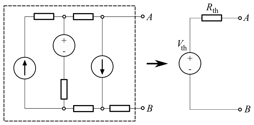
Sometimes, you don't need to analyze an entire complex circuit. You might only care about what's happening at a specific pair of terminals, like where a load resistor is connected. Thévenin's theorem is an incredibly useful tool for this. It states that any linear electrical network with two terminals can be replaced by a single voltage source ($V_{Th}$) in series with a single resistor ($R_{Th}$).

This simplified "Thévenin equivalent circuit" behaves identically to the original complex circuit from the perspective of the load. To find it:

• $V_{Th}$ is the open-circuit voltage at the terminals (the voltage when nothing is connected).
• $R_{Th}$ is the equivalent resistance at the terminals when all independent sources are turned off (voltage sources become shorts, current sources become open circuits).

Norton's theorem is the dual of Thévenin's. It states that the same complex network can be replaced by a single current source ($I_N$) in parallel with a single resistor ($R_N$).

• $I_N$ is the short-circuit current at the terminals (the current that flows when you connect a wire between them).
• $R_N$ is found the same way as $R_{Th}$ and is always equal to it ($R_N = R_{Th}$).

When a linear circuit has multiple independent sources, the superposition principle offers another way to find a particular voltage or current. It states that the total current in any branch or the total voltage across any component is the algebraic sum of the individual contributions from each source acting alone.

To apply it:

1. Pick one source and turn off all other independent sources (voltage sources become shorts, current sources become opens).
2. Calculate the desired voltage or current due to that single active source.
3. Repeat this process for every independent source in the circuit.
4. Sum the results from each step to find the final value.

These advanced techniques provide the structured framework needed to analyze any complex linear circuit you might encounter. Mastering them moves you from ad-hoc problem solving to a systematic and reliable engineering approach.