Advanced SQL Engines

Beyond Basic Queries

You've mastered SELECT, FROM, WHERE, and JOIN. You can pull data, filter it, and connect tables. But real-world data analysis often requires more. How do you find the top 3 selling products in each region? Or calculate the month-over-month growth for user sign-ups? These questions demand tools that go beyond simple data retrieval.

This is where advanced SQL engines shine. We'll explore how to structure complex logic with Common Table Expressions (CTEs), perform intricate calculations with Window Functions, and ensure your queries run efficiently on massive datasets.

Organizing Complexity with CTEs

As queries grow, they can become a tangled mess of nested subqueries. Reading them feels like deciphering a secret code. Common Table Expressions (CTEs) solve this by letting you create temporary, named result sets that you can reference later in your main query. Think of them as variables for your SQL logic.

A CTE is defined using the WITH keyword. It makes your code cleaner, more readable, and easier to debug because you can break down a complex problem into logical, sequential steps.

WITH RegionalSales AS (
  SELECT
    region,
    product_id,
    SUM(sale_amount) as total_sales
  FROM sales
  GROUP BY region, product_id
),
RankedSales AS (
  SELECT
    region,
    product_id,
    total_sales,
    RANK() OVER(PARTITION BY region ORDER BY total_sales DESC) as sales_rank
  FROM RegionalSales
)
SELECT
  region,
  product_id,
  total_sales
FROM RankedSales
WHERE sales_rank <= 3;

Notice how each CTE builds on the previous one, telling a clear story: first, calculate regional sales, then rank them, and finally, select the top 3 from the ranked results.

CTEs can also handle hierarchical data, like an organizational chart or a folder structure, through recursion. A recursive CTE has two parts: an anchor member that defines the starting point (e.g., the CEO) and a recursive member that repeatedly joins the CTE to itself until it reaches the end of the hierarchy (e.g., all direct and indirect reports).

This powerful feature lets you traverse tree-like structures, a task that is notoriously difficult with standard joins.

Analytics Without Aggregation

Standard aggregate functions like SUM() and AVG() are useful, but they have a major limitation: they collapse your data. If you use GROUP BY to find the average sale per region, you lose the details of the individual sales. How can you perform calculations across multiple rows while keeping the original row-level data?

The answer is window functionss. These functions operate on a "window" of rows related to the current row, defined by the OVER() clause. This allows you to compute running totals, moving averages, and rankings without sacrificing detail.

The OVER() clause has two main components:

PARTITION BY: This divides the rows into groups (partitions). The window function is applied independently to each partition. In our sales example, you would PARTITION BY region.
ORDER BY: This orders the rows within each partition. This is essential for functions that depend on sequence, like ranking or calculating running totals.

Let's look at a few common types of window functions.

Ranking Functions

These functions assign a rank to each row within a partition. ROW_NUMBER() assigns a unique number, while RANK() and DENSE_RANK() handle ties differently.

Name	Score	ROW_NUMBER()	RANK()	DENSE_RANK()
Alice	95	1	1	1
Bob	90	2	2	2
Carol	90	3	2	2
Dave	85	4	4	3

Notice how RANK() skips a number after a tie (rank 3 is skipped), whereas DENSE_RANK() does not. Choosing the right one depends on your specific business logic.

Time-Series and Framing Functions

For time-series analysis, LAG() and LEAD() are indispensable. LAG() lets you access data from a previous row, while LEAD() accesses data from a subsequent row. This is perfect for calculating period-over-period changes.

SELECT
  sale_month,
  monthly_revenue,
  LAG(monthly_revenue, 1) OVER (ORDER BY sale_month) as previous_month_revenue,
  (monthly_revenue - LAG(monthly_revenue, 1) OVER (ORDER BY sale_month)) / LAG(monthly_revenue, 1) OVER (ORDER BY sale_month) as mom_growth
FROM monthly_sales;

You can also define a more specific "frame" within a partition, like "the last 3 rows" or "all rows from the beginning up to the current one." This is used for calculating things like moving averages or running totals, providing powerful analytical capabilities directly within your database.

Optimizing Your Queries

Writing a query that works is one thing; writing one that runs efficiently on millions of rows is another. Poorly written queries can slow down systems and delay critical analysis. SQL query optimization is the art of making your queries faster.

Most database systems use a cost-based optimizer that generates several possible for a query and picks the one it estimates will be the cheapest (fastest). You can inspect this plan to understand how the database is actually retrieving your data. Common commands include EXPLAIN in PostgreSQL and MySQL, or EXPLAIN PLAN FOR in Oracle.

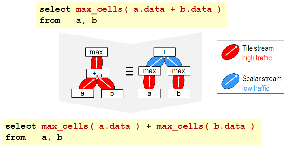
When you find a bottleneck, one of the most effective tools is indexing. An index is a special data structure that allows the database to find rows much faster, similar to the index at the back of a book. Instead of scanning the whole table (a full table scan), it can go directly to the relevant pages.

Creating an index on columns that are frequently used in WHERE clauses or JOIN conditions is a common optimization strategy. However, indexes aren't free. They take up storage space and can slow down data modification operations like INSERT, UPDATE, and DELETE. The key is to find the right balance between read performance and write overhead.

Mastering these advanced techniques—CTEs for structure, window functions for analysis, and optimization for performance—is what separates a casual SQL user from a professional data analyst. They allow you to answer complex business questions elegantly and efficiently.

Quiz Questions 1/6

What is the primary purpose of a Common Table Expression (CTE) in SQL?

Quiz Questions 2/6

Which SQL feature allows you to perform calculations across a set of table rows while still retaining the original row-level data?

Advanced Data Analytics Professional