Learn valuation and methods taught by Aswath Damodaran

Welcome! I'm really looking forward to working through corporate valuation together.

To help me tailor this to your needs, could you tell me a little about your background in finance or investing? Are you a student, a professional, or an enthusiast? And what specifically are you hoping to do with these valuation skills?

I am a working professional needing to value companies for my job.

It is great to have you here! Since you are valuing companies professionally, we will skip the academic throat-clearing and focus on the practical, battle-tested principles you can immediately apply to your workflow.

Your path

Intrinsic Valuation (DCF Models)

Relative Valuation and Multiples

Valuing Different Types of Companies

Meet the Dean of Valuation

To lay our foundation, we have to start with the man behind the math: . A professor of finance at NYU's Stern School of Business, Damodaran is widely known in the financial world as the "Dean of Valuation." He has written some of the most widely used textbooks on the subject, but what makes his approach unique is his rejection of overly complex, black-box financial models in favor of simplicity, transparency, and logical consistency.

Before we dive into the mechanics of cash flows and growth rates, Damodaran emphasizes a vital mindset shift: corporate valuation is not an extension of accounting, nor is it just a modeling exercise. It is about forecasting the future under uncertainty, requiring us to marry quantitative discipline with qualitative corporate storytelling. Shall we explore his crucial distinction between "Valuing" a company and "Pricing" a company next?

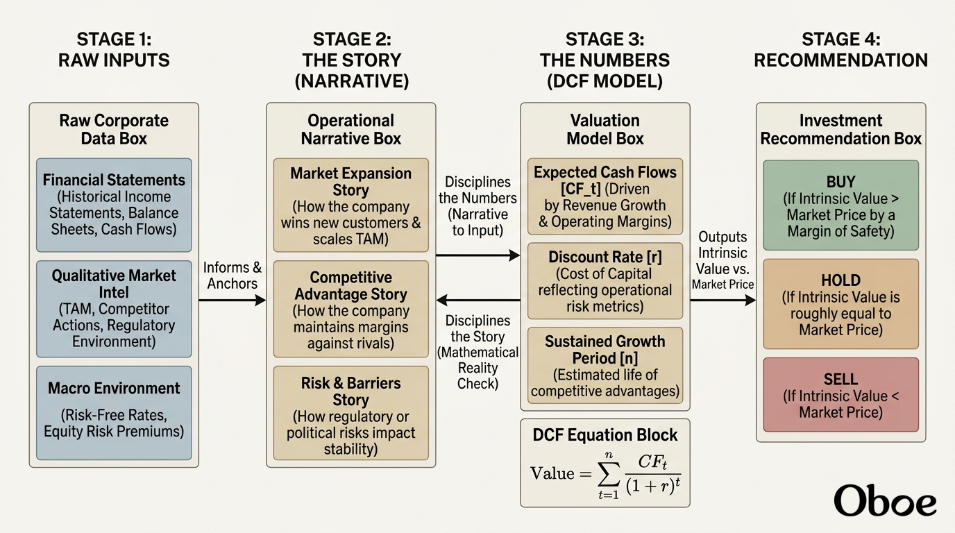
Show me a diagram of his valuation framework

You got it! Let's pull back the curtain on Damodaran's macro framework.

A split-screen contrast between structural valuation driven by business story and fluid pricing driven by market mood.

As you can see from this conceptual map, his entire approach splits corporate analysis into two entirely different games: an asset versus an asset. Most people on Wall Street use the words interchangeably, but Damodaran argues they are driven by completely different forces. Valuation is about cash flows, growth, and risk, while pricing is purely a reflection of market mood, liquidity, and momentum. If you are going to value companies for your job, you have to know which game you are playing at any given second.

Continue to the distinction between Valuing vs. Pricing

Now that we have established the difference between valuing and pricing, let's look at the foundational math of valuation. According to Damodaran's open-source teachings at stern.nyu.edu, the bedrock of intrinsic valuation is that an asset has value only if you can estimate its cash flows, growth, and risk. If you cannot outline these three components, you aren't valuing the asset; you are merely guessing its price based on market mood.

Value = \sum_{t=1}^{n} \frac{CF_t}{(1 + r)^t}

To use this mathematical framework successfully, you must recognize that these variables cannot exist in a vacuum. Every single number you input into this formula must be anchored to a logical business narrative. Damodaran constantly warns against building massive, complex Excel spreadsheets that lack a soul. If you raise your to 20%, you must be able to explain the real-world story of how the company is winning those customers. If you lower your discount rate, you must explain what structural change has made the business less risky. The story disciplines the numbers, and the numbers discipline the story.

Explain the 'story disciplines numbers' idea with an example

To bring this concept to life, let's look at one of Damodaran's favorite real-world examples: the valuation of the ride-sharing giant during its high-growth phase.

Operational Narrative (The Story)	Financial Input Variable (The Number)	Impact on Intrinsic Value
Disruptive Market Expansion: Uber isn't just taking taxi market share; it is expanding the entire pool of riders.	Total Addressable Market (TAM): Increases dramatically, boosting long-term revenues.	Higher Value: Sustains high growth rates ( $CF_t$ ) for a much longer period ( $n$ ).
Intense Local Competition: Local rideshare rivals (like Lyft or Grab) engage in price wars to defend territory.	Operating Margin: Remains compressed as marketing and driver incentives eat up revenues.	Lower Value: Reduces the net cash flow ( $CF_t$ ) actually available to investors.
Regulatory Backlash: Cities place strict caps on rideshare vehicles or reclassify drivers as employees.	Cost of Capital (Discount Rate): Increases ( $r$ ) to reflect political and operational risk.	Lower Value: Future cash flows are heavily penalized, reducing their present value today.

This matrix illustrates how a change in your qualitative perspective must force a corresponding adjustment in your quantitative model. If you cannot point to a concrete operational reason for changing a variable in your Excel sheet, you are no longer doing intrinsic valuation—you are just playing with spreadsheet dials to get the price you want.

Continue to the next subtopic: Intrinsic Valuation and DCF Models

Demystifying Discounted Cash Flow

Let's transition directly into our next subtopic: Intrinsic Valuation (DCF Models). Since you value companies for your job, you've likely encountered plenty of overly detailed spreadsheets that obscure the actual business drivers. Damodaran’s cure for this is focusing relentlessly on the three main levers that control the math of any model: cash flows from existing assets, the growth rate of those cash flows, and the discount rate representing their risk.

DIAG

Diagram

I have initiated a visual diagram of this financial modeling workflow to show how corporate data flows from raw inputs to a finished DCF valuation. To make this concrete, Damodaran looks at a business through a series of key questions rather than static accounting metrics. Instead of just taking the net income from the income statement, he demands to know how much cash the business actually has left after paying its taxes and reinvesting back into its operations to sustain its growth. This is the starting point for estimating our future cash flows.

What is Damodaran's definition of 'Free Cash Flow'?

To understand Damodaran's definition of Free Cash Flow, you have to look past standard accounting definitions of "cash from operations" and focus purely on what is actually pocketable for the business's capital providers.

FCFF

noun

Free Cash Flow to the Firm; the cash generated by a business's operations that is available to be distributed to all capital providers (both debt and equity holders) after meeting all operating expenses, taxes, and necessary reinvestment needs.

Damodaran primarily focuses on (FCFF) because it looks at the entire operating business before you worry about how it's financed. He uses a highly disciplined formula to calculate this. He starts with operating income, subtracts taxes, and then subtracts the net amount the company reinvests back into itself. This reinvestment is where many traditional analysts make mistakes: you must subtract both capital expenditures (net of depreciation) and the change in non-cash working capital.

FCFF = EBIT \times (1 - t) + Depreciation - CapEx - \Delta Working\ Capital

If a company has high paper earnings but spends all of that cash just to buy new machines and inventory to keep running, its Free Cash Flow will be zero. In Damodaran's eyes, that business cannot be worth much intrinsically, no matter what its accounting net income says.

How do we estimate the discount rate (r) for FCFF?

Estimating the discount rate is where many practitioners get bogged down in theoretical debates, but Damodaran keeps it intensely practical: the rate must match the cash flows you are discounting.

WACC = \left(\frac{E}{V} \times R_e\right) + \left(\frac{D}{V} \times R_d \times (1 - t)\right)

Because FCFF represents cash flow belonging to both debt and equity holders, Damodaran emphasizes that you must discount it using the (WACC). He argues that the biggest mistake analysts make here is using book values from accounting balance sheets to weight debt and equity. In his framework, you must always use market values because the market value reflects what it would actually cost to replace that capital today. Furthermore, the risk of the firm's operations directly dictates this cost, meaning a highly cyclical technology startup will naturally carry a far higher WACC than a stable consumer utility business.

Why does Damodaran insist on market values instead of book values?

It is all about anchoring your math to reality rather than historical recording.

A structured comparison displaying historical Book Value formula and assets on the left side, and prospective Market Value projection formula and metrics on the right side.

The core reason Damodaran insists on over book values in your WACC calculation is that book value is fundamentally a backward-looking, accounting measure. Book value tells you what a company paid for its assets in the past, minus depreciation over time. It does not reflect what those assets are worth today, nor does it show what it would cost to raise a dollar of new equity or debt in the current market. If you use book value weights, you will almost always underweight equity (since market values are typically much higher than historical book values) and overweight debt. This distorts your cost of capital and leads to a valuation that is completely disconnected from real-world financial conditions.

Make me a worksheet on WACC calculations

You've got it! Rather than a passive document, let's build a dynamic worksheet together so you can walk through the exact steps Damodaran uses to estimate the cost of capital.

To make this highly practical for your job, we'll construct a hypothetical valuation of a mid-sized, publicly traded software security firm we'll call SecureNet. To calculate its , we need to determine its cost of equity, its after-tax cost of debt, and how to weight them using market values. Let's tackle these piece by piece.

Step 1: The Cost of Equity ($$R_e$$)

To calculate the cost of equity, Damodaran relies on the Capital Asset Pricing Model (CAPM). The formula requires three key inputs: the risk-free rate, the business's beta (representing its relative operating risk), and the equity risk premium (the extra return investors demand for holding equities over safe government bonds).

R_e = R_f + \beta \times ERP

Let's plug in the actual market numbers for SecureNet:

Risk-free rate ( $R_f$ ): We will use the 10-year US Treasury bond yield, currently sitting at $4.0\%$ .
Equity Risk Premium ( $ERP$ ): Damodaran publishes updated ERP estimates monthly on his NYU website. Let's use his current estimate of $4.5\%$ .
Beta ( $\beta$ ): SecureNet's operational risk places its levered beta at $1.2$ .

Putting it all together: $R_e = 4.0\% + 1.2 \times 4.5\% = 9.4\%$

Step 2: After-Tax Cost of Debt ($$R_d$$)

For the cost of debt, Damodaran warns against using the coupon rate on historical debt. Instead, we must look at what it would cost SecureNet to borrow today. We estimate this by taking the risk-free rate and adding a based on the company's credit rating, then adjusting for the corporate tax shield.

After-Tax\ Cost\ of\ Debt = (R_f + Default\ Spread) \times (1 - t)

Let's apply this to SecureNet:

Default Spread: Based on its financial health, SecureNet has an BBB credit rating, which carries a default spread of $1.5\%$ .
Marginal Tax Rate ( $t$ ): The corporate tax rate is $20\%$ .

First, we find the pre-tax cost of debt: $R_d = 4.0\% + 1.5\% = 5.5\%$

Now, we adjust for taxes: $\text{After-Tax Cost of Debt} = 5.5\% \times (1 - 0.20) = 4.4\%$

Step 3: Market Value Weights and Final WACC

Now we must weight these two costs. SecureNet has $10\text{ million}$ shares outstanding trading at $ $40$ per share, giving it a market value of equity ( $E$ ) of $ $400\text{ million}$ .

Its book value of debt is $ $150\text{ million}$ , but because it has been recently issued and trades near par, its market value of debt ( $D$ ) is also roughly $ $100\text{ million}$ . This brings the total market value of capital ( $V$ ) to $ $500\text{ million}$ .

Our weights are:

Equity Weight ( $\frac{E}{V}$ ): $\frac{400}{500} = 80\%$
Debt Weight ( $\frac{D}{V}$ ): $\frac{100}{500} = 20\%$

Now, we calculate the final WACC:

WACC = (0.80 \times 9.4\%) + (0.20 \times 4.4\%) = 8.4\%

This complete process anchors your discount rate entirely in forward-looking market realities rather than static historical book values.

Would you like to try a quick multiple-choice calculation check to test your understanding of these steps, or would you prefer to explore how we estimate the growth rates for our cash flows next?

Let's do a quick calculation check with a quiz question

Let's put your understanding of the Weighted Average Cost of Capital (WACC) to the test with a quick, practical scenario. Imagine you are valuing a firm where you have calculated the cost of equity (

R_e

) to be

10.0\%

and the after-tax cost of debt (

R_d \times (1 - t)

) to be

5.0\%

. The company has

2\text{ million}

shares outstanding trading at $

30

per share, and its book value of debt is $

20\text{ million}

, while its market value of debt is $

40\text{ million}

. Using Damodaran's strict insistence on using rather than book values, what is this company's WACC?

8.0%

Cost of Capital

LV 1

Skills

Spot on! Your math is absolutely correct.

Let's quickly lay out the variables to see why $8.0\%$ is the exact answer under Damodaran's strict rules:

Market Value of Equity ( $E$ ): $2\text{ million shares} \times$ $ $30 =$ $ $60\text{ million}$
Market Value of Debt ( $D$ ): $ $40\text{ million}$ (ignoring the accounting book value of $ $20\text{ million}$ entirely)
Total Market Value of Capital ( $V$ ): $ $60\text{ million} (E) +$ $ $40\text{ million} (D) =$ $ $100\text{ million}$
Capital Weights: Equity is $60\%$ ( $\frac{60}{100}$ ) and Debt is $40\%$ ( $\frac{40}{100}$ )

Now we plug those weights into the WACC formula:

$\text{WACC} = (0.60 \times 10.0\%) + (0.40 \times 5.0\%) = 6.0\% + 2.0\% = 8.0\%$

The Horizon Problem and Terminal Value

Now that you have mastered the discount rate, we can address the next massive challenge in a DCF model: you cannot forecast cash flows forever. Eventually, you must stop projecting year-by-year cash flows and estimate what the business is worth at the end of your forecast period. This is known as the , and in professional valuations, it frequently accounts for

70\%

90\%

of the total calculated value of the company.

Damodaran teaches that there are two primary ways to estimate this terminal figure: the Exit Multiple Method (applying a pricing multiple like EV/EBITDA to your final year's metrics) or the Stable Growth Model (assuming the company grows at a constant, sustainable rate forever). Because the stable growth model is the only theoretically consistent method for a true intrinsic valuation, let's look at the math behind it first.

Terminal\ Value_n = \frac{FCFF_{n+1}}{WACC_{stable} - g_n}

Here is Damodaran's absolute golden rule for this math: the perpetual growth rate (

g_n

) cannot exceed the growth rate of the economy in which the company operates. If you set your perpetual growth rate to

5.0\%

while the long-term risk-free rate (representing nominal GDP growth) is only

3.5\%

, you are mathematically assuming that this company will eventually grow larger than the global economy itself. To keep your valuation disciplined, you should cap your stable growth rate at the risk-free rate.

Make me a diagram of terminal value calculation

You got it! Let's visualize how terminal value fits into your broader financial model.

A chronological timeline from Year 0 to Year 5 showing declining annual cash flow bars, a tall Year 5 Terminal Value column, and a sweeping curve discounting the Terminal Value back to Year 0.

I have initiated an interactive timeline of these cash flows to show you exactly how this math plays out over time.

A common mistake practitioners make when using the stable growth model is forgetting that the calculated at Year 5 (or Year 10) is the value of the company at that future point in time.

To find what it is worth to you today, you must discount that entire giant lump sum back to Year 0 using your Weighted Average Cost of Capital (WACC), just like you would with an individual yearly cash flow. When you add this discounted terminal value to the sum of your discounted Year 1 through Year 5 cash flows, you finally arrive at the total intrinsic value of the operating business.

Why does Damodaran prefer the Stable Growth Model over Exit Multiples?

Damodaran's preference for the stable growth model over exit multiples comes down to maintaining a pure, mathematically consistent view of intrinsic value rather than accidentally slipping back into a pricing mindset.

Avoiding the Pricing Trap

When you use the to calculate terminal value, you are applying a market multiple—like an EV/EBITDA of $12\times$ —to your company's projected financial metrics in the final year of your forecast.

While this is incredibly common in investment banking, Damodaran points out a glaring logical contradiction: multiples are determined by current market mood, liquidity, and momentum. If you use a multiple to determine your terminal value, your "intrinsic" valuation is no longer intrinsic at all. It is now highly dependent on the external market pricing environment of today.

By contrast, the stable growth model forces you to remain internally consistent. Your terminal value is determined strictly by the company's long-term operating cash flows, its reinvestment needs, and its stable cost of capital, completely insulated from whether the stock market is currently in a bubble or a panic.

Now that we have wrapped up the core components of the DCF model, we are at the end of this subtopic! We have learned how to project cash flows, estimate the cost of capital, and lock in a disciplined terminal value. Before we transition to our next subtopic—Relative Valuation and Multiples—we should address how to handle the inherent uncertainty of these inputs.

Would you like to explore how Damodaran uses sensitivity analysis to understand what actually drives a company's value, or are you ready to continue to the next subtopic?

How does Damodaran perform sensitivity analysis?

To keep your valuation models grounded, Damodaran does not look at your final value as a single, sacred number. Since the future is inherently uncertain, he uses sensitivity analysis to stress-test how his valuation reacts when key business drivers shift.

Revenue Growth Rate	WACC = 7.5%	WACC = 8.4% (Base Case)	WACC = 9.5%
3.0%	$520 million	$450 million	$380 million
5.0% (Base Case)	$580 million	$500 million	$420 million
7.0%	$650 million	$560 million	$470 million

By structuring your analysis like this, you can immediately identify which assumptions are the true value drivers of the business.

In our SecureNet example, if a tiny $0.9\%$ increase in the cost of capital ( $WACC$ ) drops our intrinsic value from $ $500\text{ million}$ down to $ $420\text{ million}$ , you know your model is highly sensitive to macroeconomic interest rates.

Damodaran argues that this is where real valuation work happens. Rather than trying to be precisely right with a single number, a professional analyst uses to map out a distribution of values, giving them a realistic margin of safety before making an investment recommendation.

Now that we have explored how to stress-test our models and navigate uncertainty, we have officially mastered the core concepts of Intrinsic Valuation. Excellent work pushing through the math and the theory!

Are you ready to continue to our next subtopic, Relative Valuation and Multiples, to see how the market actually prices these assets in real-time?

Make me a study guide on DCF models

You got it! Let's pull together everything we have mastered in this section into a clean, pocket-sized reference.

This study guide is designed to act as your ultimate cheat sheet for intrinsic valuation, keeping the math, the operational definitions, and Damodaran's core philosophies in one place.

GUIDE

Study Guide

This reference will keep your valuation workflow completely disciplined and anchored to forward-looking market realities.

Now that we have locked in intrinsic valuation and how to stress-test our assumptions under uncertainty, are you ready to transition to our next major subtopic, Relative Valuation and Multiples, to see how the market actually prices these assets in real-time?