Intermediate Data Structures and Algorithms Mastery
Efficiency and Performance Analysis
Beyond Big O Notation
You're likely familiar with Big O notation as a way to describe an algorithm's worst-case performance. It tells us the upper bound on how runtime or memory usage grows with the input size. While incredibly useful, Big O is only one part of the story. To make informed engineering decisions, especially when building scalable systems, we need a more complete vocabulary for performance analysis.
Thinking in terms of upper bounds, lower bounds, and average cases allows us to understand the full performance profile of our code, not just the worst-case scenario.
The Full Picture: Ω and Θ
Big O describes the ceiling, but what about the floor? That's where Big Omega (Ω) comes in. Big Omega notation describes the best-case scenario, or the lower bound on an algorithm's performance. It guarantees that an algorithm will take at least a certain amount of time.
When an algorithm's best-case and worst-case performance scale in the same way, we can use Big Theta (Θ) notation. A Θ bound is a tight bound; it tells us that the algorithm's growth rate is sandwiched between two constants multiplied by the same function. Essentially, it describes the precise growth rate.
| Notation | Name | Describes | Analogy |
|---|---|---|---|
| O(f(n)) | Big O | Upper Bound | "This task will take at most this long." |
| Ω(f(n)) | Big Omega | Lower Bound | "This task will take at least this long." |
| Θ(f(n)) | Big Theta | Tight Bound | "This task will take exactly this long, relatively speaking." |
Consider searching for an item in an unsorted array of size n. In the best case, the item is the very first one you check. This is an Ω(1) operation. In the worst case, it's the last item, or not in the array at all, requiring you to check all n elements. This is an O(n) operation. Since the upper and lower bounds are different, we cannot describe this search with Θ notation.
However, iterating over every element in an array to, say, sum them up will always require visiting each of the n elements. The best and worst cases are identical. Therefore, this operation is Θ(n).
Amortized Analysis and Dynamic Arrays
Some data structures have operations that are usually fast, but occasionally very slow. A dynamic array (like Python's list or C++'s std::vector) is a perfect example. Adding an element is typically an O(1) operation. But what happens when the underlying array is full?
The data structure must allocate a new, larger array (often double the size), copy all the old elements over, and then add the new one. This single append operation is slow—O(n), where n is the current number of elements. If we only looked at the worst-case, we'd think dynamic arrays are inefficient for adding data. This is where amortized analysis gives us a more practical perspective.
Amortized analysis averages the cost of expensive operations over the entire sequence of operations. While a single resize is O(n), it happens so infrequently that its cost is spread out, or amortized, over the many cheap O(1) appends. The result is that the amortized cost of an append operation on a dynamic array is O(1). This explains why they are so fast and effective in practice, even with occasional costly resizes.
The Space-Time Tradeoff
In system design, you rarely get something for nothing. One of the most fundamental trade-offs is between time (computation speed) and space (memory usage). You can often make an algorithm faster by using more memory, or reduce memory consumption at the cost of slower execution.
A classic example is caching. Storing pre-computed results in a cache (using more memory) allows for near-instant retrieval later, saving the time it would take to compute them again.
This principle extends beyond caching. Memoization in recursive algorithms, for instance, stores the results of function calls to avoid redundant computations. This uses extra space for the lookup table but can turn an exponential-time algorithm into a linear-time one. When designing systems, engineers constantly make decisions about where to sit on this spectrum, balancing server costs (memory) with user experience (speed).
Choosing the right balance depends entirely on the constraints of the system. For a mobile app on a device with limited RAM, optimizing for space might be the priority. For a high-frequency trading system where microseconds matter, developers will use as much memory as needed to achieve maximum speed.
The Memory Hierarchy and Performance
Asymptotic complexity doesn't account for the physical realities of hardware. An algorithm that is theoretically fast can be slow in practice if it doesn't work well with modern computer architecture. A key concept here is the memory hierarchy and its impact on performance.
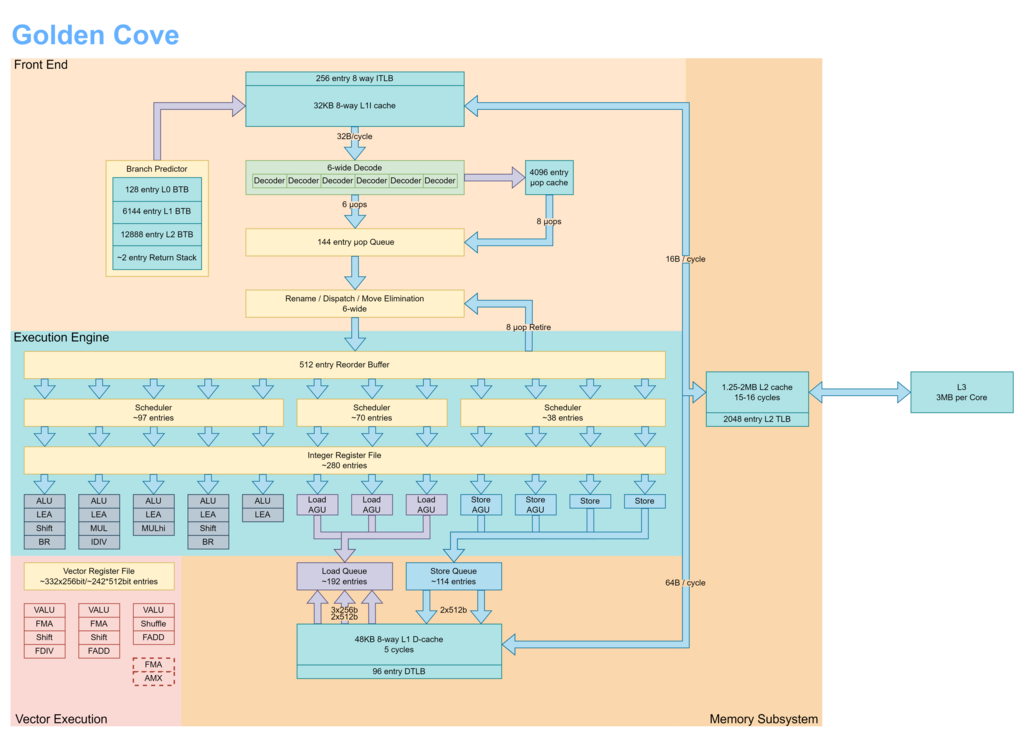
Computers have different levels of memory, each with different speeds and sizes:
- CPU Registers: Fastest, but tiny.
- L1/L2/L3 Caches: Very fast, located on the CPU, but still small.
- RAM (Main Memory): Much larger, but significantly slower than caches.
- Disk Storage (SSD/HDD): Enormous, but orders of magnitude slower than RAM.
Accessing data from RAM is far more expensive than accessing it from a CPU cache. Algorithms that exhibit good cache locality—meaning they access memory locations that are close to each other in sequence—tend to be much faster in the real world. When the CPU requests data from a memory address, it also pulls in a chunk of adjacent memory (a "cache line") into the super-fast cache. If the next piece of data the algorithm needs is already in that cache line, the access is nearly instantaneous. This is a cache hit. If it's not, the CPU must stall and wait for data to be fetched from RAM, a much slower process called a cache miss.
This is why iterating through a contiguous array is often faster than traversing a linked list, even if they both store the same number of elements and have the same Big O complexity for iteration. The array's elements are stored together in memory, leading to excellent cache locality.
Let's put everything we've learned together. Now, test your knowledge.
Which notation provides a tight bound on an algorithm's growth rate, describing its performance when the best-case and worst-case scenarios scale identically?
Consider an algorithm that iterates through every element of an array of size n to find the maximum value. What is the most precise asymptotic notation for this operation?
Understanding these deeper layers of performance analysis moves you from simply writing code that works to engineering solutions that are efficient, scalable, and tailored to real-world hardware constraints.