Data Science Foundations in Practice
Data Preprocessing Strategies
Beyond Cleaning: Strategic Preprocessing
You already know that raw data is messy. Fixing obvious errors like typos or impossible values is data cleaning. Data preprocessing, however, is a different beast. It's the strategic process of transforming your clean data into the optimal format for a machine learning model.
Think of it like this: cleaning is fixing a damaged ingredient, while preprocessing is carefully chopping, measuring, and combining ingredients to bake a perfect cake. The choices you make here directly influence your model's ability to learn and make accurate predictions.
Data cleaning and preprocessing are fundamental steps in the data science process.
Handling Missing Data Intelligently
Replacing missing values with the mean or median is a quick fix, but it often overlooks the relationships between variables. For more sophisticated models, we need smarter imputation techniques that leverage the dataset's underlying structure.
Imputation
noun
The process of replacing missing data with substituted values.
One powerful method is K-Nearest Neighbors (KNN) Imputation. Instead of looking at the entire column, this technique finds the 'k' most similar data points (the "neighbors") to the one with the missing value. It then uses the values from these neighbors, often by averaging them, to fill in the blank.
Imagine trying to guess a person's favorite movie. A simple approach might be to guess the most popular movie overall. A KNN approach would be to find people with similar tastes in other movies and guess based on what they like. It's a more personalized, context-aware estimate.
Another advanced method is Iterative Imputation. This approach models each feature with missing values as a function of all other features. It works in rounds: it makes an initial guess for each missing value, then cycles through the features, predicting the missing values in one feature based on all the others. It repeats this process, refining its predictions each round until the estimates stabilize.
This is like a detective solving a case with partial clues. They form an initial theory, then use that theory to re-evaluate each piece of evidence, which in turn refines the theory. This continues until a coherent story emerges.
Encoding and Scaling
Models need numbers, not text. Converting categorical features into a numerical format is called encoding. You're likely familiar with One-Hot Encoding, which creates a new binary column for each unique category. This is great for features with a few categories, like 'Color' (Red, Green, Blue).
But what about high-cardinality features, like 'Zip Code' or 'User ID', which can have thousands of unique values? One-Hot Encoding would create an unmanageable number of new columns. This is where Target Encoding comes in.
Target Encoding replaces each category with the average value of the target variable for that category. For example, if you're predicting customer churn, the category 'New York' would be replaced by the average churn rate of all customers from New York. This is a powerful way to capture information in a single feature, but it must be used carefully to avoid overfitting.
| Method | Best For | Downside |
|---|---|---|
| One-Hot Encoding | Low-cardinality features | Creates too many columns for high-cardinality features |
| Target Encoding | High-cardinality features | Can lead to overfitting if not implemented carefully |
After encoding, we often need to scale our numerical features. Many models are sensitive to the scale of the input data. For example, a feature ranging from 0 to 100,000 will have a much larger influence than a feature ranging from 0 to 1. StandardScaler is a common choice; it rescales data to have a mean of 0 and a standard deviation of 1.
However, StandardScaler is sensitive to outliers. A few extreme values can skew the mean and standard deviation, warping the scaled data. When you suspect your data has significant outliers, RobustScaler is a better choice. It uses the median and interquartile range, making it—as the name implies—robust to the influence of outliers.
The Danger of Data Leakage
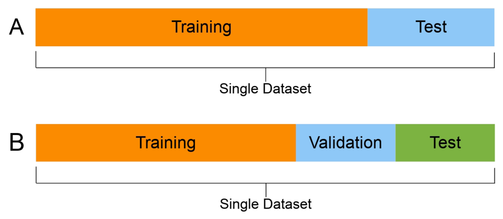
Data leakage is one of the most insidious problems in machine learning. It happens when information from your test set accidentally 'leaks' into your training process. This gives you an overly optimistic view of your model's performance, which will crumble when it sees truly new data.
A classic example occurs during scaling. If you calculate the mean and standard deviation for scaling from your entire dataset before splitting it into training and testing sets, you've committed a data leak. The training process has now been influenced by information from the test set. The model 'knows' something about the data it's supposed to be tested on.
The golden rule: Never use any information from your test set to preprocess your training set. All calculations for scaling, imputation, or encoding should be derived only from the training data.
How do you prevent this? The best practice is to use pipelines. A pipeline chains together multiple preprocessing steps (like imputation, encoding, and scaling) into a single object. When you train the pipeline, it learns the parameters for each step (e.g., the mean for scaling) only from the training data. Then, when you use the pipeline to transform the test data, it applies those same learned transformations without recalculating anything.
This enforces a strict separation between training and testing, preventing data leakage and making your workflow cleaner and more reproducible.
Let's review what we've learned.
What is the primary difference between data cleaning and data preprocessing?
You need to impute missing 'household_income' values. You suspect income is strongly related to other features like 'neighborhood' and 'job_title'. Which imputation strategy would be most effective at capturing these relationships?
With these strategies, you can move beyond simple cleaning and prepare datasets that are truly ready for modeling, ensuring your results are both accurate and reliable.