Your analysis is only as good as your data. In the real world, data rarely arrives clean. You’ll get reports from different departments, exports from various systems, and manually entered spreadsheets. The result is often a mess of inconsistent formats, extra spaces, and structural differences that make analysis impossible.

Instead of spending hours manually cleaning this data, you can automate the process using Power Query (now called 'Get & Transform' in the Data tab). Think of it as a repeatable recipe for your data. You show it once how to clean and combine your sources, and it remembers every step. The next time you get updated files, you just hit 'Refresh'.

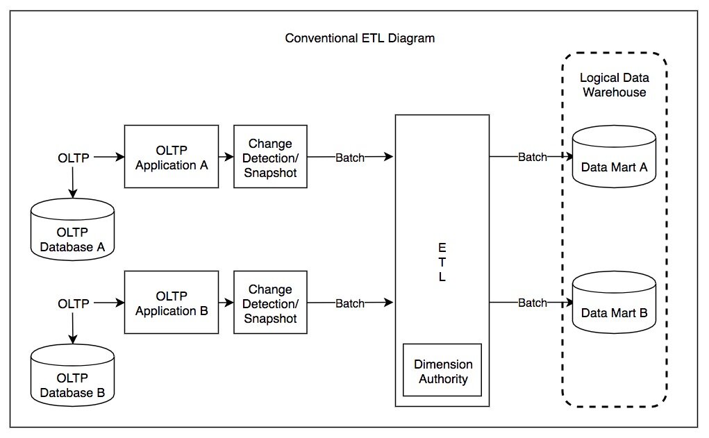
Let’s say you have two monthly sales reports. They have similar information but are formatted differently. One has extra spaces in the product names, and the other uses a mix of DD-MM-YYYY and MM/DD/YY date formats.

Using Power Query, you would:

1. Extract: Load both tables into the Power Query editor.
2. Transform: Use the 'Trim' function to remove leading and trailing spaces from the product names. Then, you'd select the date columns and set a consistent data type, letting Power Query automatically parse the different formats.
3. Load: Combine (or 'Append') the two cleaned tables into a single, master table, and load it into a new worksheet. From that point on, any new data added to your source files gets cleaned and added to the master table with a single click.

Once your data is clean, you can start building dynamic models. While VLOOKUP is a classic, modern Excel offers XLOOKUP, a far more flexible and robust function. Unlike VLOOKUP, XLOOKUP can look to the left of the lookup column, return entire rows or columns, and has a built-in 'if not found' argument, eliminating the need to wrap it in an IFERROR function.

Another powerful technique is creating dependent dropdown lists using Data Validation. This is where the selection in one list filters the options available in another. For example, a user first selects a region ('North', 'South'), and a second dropdown list automatically populates with only the cities from that region. This prevents data entry errors and makes your spreadsheets much more user-friendly. You can achieve this by combining Data Validation with functions like FILTER or the older, more complex INDIRECT.

Standard Pivot Tables are fantastic for summarizing data, but they struggle with millions of rows and can't easily create relationships between different tables. This is where Power Pivot comes in. It's a data modeling engine that allows you to work with massive datasets and connect multiple tables, just like in a database.

The true power of this feature is unlocked with DAX (Data Analysis Expressions). DAX is a formula language used to create custom calculations within Power Pivot. While it looks similar to Excel formulas, it operates on entire tables and columns rather than individual cells.

You can create two types of calculations:

• Calculated Columns: These add a new column to your data model, with a value calculated for each row. For example, [Price] * [Quantity] to create a Total Sale column.
• Measures (or Calculated Fields): These are aggregated calculations that respond to the context of your Pivot Table. For example, SUM([Total Sale]) creates a measure that will correctly calculate the sum of sales no matter how you slice your data—by region, by month, or by product.

Measures are more efficient and flexible than calculated columns for aggregations. They don't store extra data and calculate on the fly, making your analysis fast and dynamic.

Many reporting tasks are repetitive: download the latest data, clean it up, refresh a Pivot Table, and email the summary. You can automate this entire workflow using Macros. A macro is a recording of your actions in Excel that you can play back at any time.

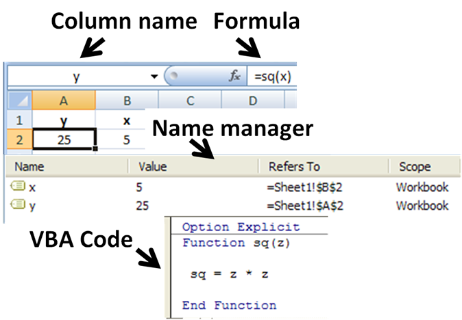
You can start by using the Macro Recorder (found in the 'Developer' tab) to record your steps. For instance, you could record the action of refreshing all data connections and then formatting a report table. Once recorded, you can assign the macro to a button on your worksheet. Clicking the button executes all the recorded steps in an instant.

For more complex logic, you can edit the recorded macro's code in the Visual Basic for Applications (VBA) editor. This opens up a world of possibilities, from automatically generating and emailing PDF reports to creating custom user forms for data entry.

Now you have the tools to not only clean and analyse data but also to create dynamic, automated, and error-proof reports.