Imagine trying to find the average height of every adult in a country. Measuring everyone is impossible, so you take a sample, say 1,000 people, and calculate their average height. You get a single number: 175 centimeters. This is a point estimate—a single value used to estimate a population parameter.

The problem? It's almost certainly wrong. The true average height of the entire population might be 175.1 cm, 174.98 cm, or something else entirely. Your point estimate is precise, but its chances of being exactly correct are virtually zero. It's like throwing a dart at a number line and expecting it to land exactly on the true value. Sampling variability ensures that every sample will produce a slightly different mean.

Instead of aiming for an exact number we'll surely miss, we can define a range of plausible values. This is called an interval estimate. It’s like saying, “I’m pretty confident the true average height is somewhere between 174 cm and 176 cm.” This approach acknowledges the uncertainty inherent in sampling and gives us a more useful result.

To build a useful interval, we need a way to measure the variability of our sample estimates. You already know that the standard deviation measures the spread in a population or a single sample. But what about the spread of sample means themselves? If we took 100 different samples of 1,000 people, we'd get 100 slightly different sample means. How much would those means vary?

This is measured by the standard error (SE). It’s the standard deviation of the sampling distribution of a statistic, like the sample mean. The Central Limit Theorem tells us that this sampling distribution is approximately normal for large samples. The standard error is our key to quantifying the uncertainty of our point estimate.

For a sample mean, the formula for the standard error is straightforward. It's the population standard deviation ($\\\sigma$) divided by the square root of the sample size ($n$).

In practice, we rarely know the true population standard deviation $\\\sigma$. So, we estimate it using the sample standard deviation, denoted as $s$.

The same logic applies to proportions. If you want to estimate the proportion of people who prefer a certain candidate, the standard error for a sample proportion ($p$) is calculated differently, but serves the same purpose.

The standard error is the foundation, but it's not the whole story. To create our interval, we multiply the standard error by a critical value from a probability distribution (often a z-score for large samples). This product is called the margin of error. It's the 'plus or minus' value we add to and subtract from our point estimate to create the interval.

The full interval estimate, also known as a confidence interval, is constructed like this:

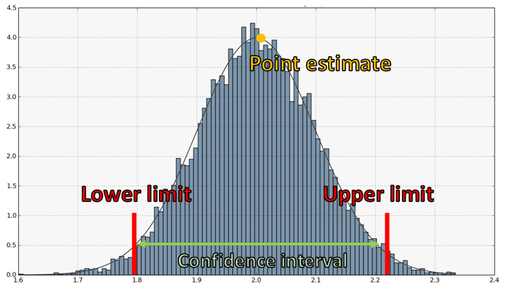
This range gives us a set of plausible values for the true population parameter. Instead of making a single, precise claim that's bound to be wrong, we create a more honest and useful range that reflects the reality of sampling.

Ready to check your understanding?

By moving from a single point to an interval, we build a more robust picture of what the true population parameter might be, fully acknowledging the uncertainty that comes with working with samples.