Welcome! I'm excited to help you master assembly language. Before we dive into the core concepts of CPU architecture and memory models, I'd love to tailor our path to your exact goals.

Given your strong background in advanced computer science, which specific CPU architecture would you like us to focus on, and what is your primary motivation for learning assembly?

Excellent choice. Focusing on x86-64 is perfect for operating system development and squeezing out every ounce of hardware performance. Let's look at how our learning journey is mapped out to get you comfortable at the bare-metal level.

The x86-64 CPU and Registers

• rax: The full 64-bit register.
• eax: The lower 32 bits of rax.
• ax: The lower 16 bits of rax.
• al: The lower 8 bits of rax.

I've started generating an interactive diagram to help you visualize how these nested registers map onto the physical hardware. Notice how modifying the smaller 32-bit eax register actually affects the lower half of the 64-bit rax register.

While all 16 of our general-purpose registers can hold arbitrary 64-bit values, the x86-64 calling conventions assign specialized roles to several of them to keep software running predictably.

Because you are diving into low-level performance optimization and OS development, keeping track of these default register roles will help you write clean assembly and correctly interface with the BIOS or kernel.

Let's do a quick check-in on this before we look at volatile and non-volatile classifications. Imagine you are executing a function that performs a quick calculation and needs to pass its final 64-bit integer output back to a calling C function. Which register should hold that output?

Spot on. rax is the designated return value register under x86-64 calling conventions, making it the gateway for functions to send data back up the chain.

Now let's talk about register ownership. When functions call other functions, who is responsible for keeping register values safe? To prevent data from being accidentally overwritten, x86-64 divides general-purpose registers into two categories:

• Volatile (Caller-Saved) Registers: Think of these as public scratchpads. The function being called is free to overwrite them without warning. If the calling function has important data in a volatile register (like rax, rcx, or rdx), it must save that data to the stack before making the call, and restore it afterward.
• Non-Volatile (Callee-Saved) Registers: These are private workspaces. If a function wants to use one of these registers (like rbx or rsp), it must back up the original value first and restore it before returning, leaving it exactly how it found it.

This classification is a cornerstone of writing reliable kernel code, ensuring that your context switches or device drivers don't unexpectedly mangle application state.

The Instruction Pointer

While general-purpose registers hold your variables and memory addresses, there is one highly specialized register that coordinates the entire show: the instruction pointer, or rip in x86-64.

Unlike general-purpose registers, you cannot directly write values to rip using standard instruction operations like a move instruction. Instead, the CPU automatically updates rip as it steps through machine instructions. When you execute a jump, call, or return, the CPU modifies this pointer under the hood to alter the execution flow.

Let's put your understanding of these x86-64 registers to the test. Since you are developing low-level operating system code, keeping track of register volatile states and control pointers is absolutely critical to avoid catastrophic system crashes.

That is absolutely correct. The instruction pointer, rip, is managed directly by the hardware's internal execution cycle, updating automatically as it fetches each instruction.

You have fully mastered the fundamentals of registers and CPU architecture. This solid foundation is going to make writing actual code much more intuitive. We are now ready to step up our game and move to the second phase of our journey: looking at the actual code syntax and basic instructions that let us move and manipulate data.

Welcome to Assembly Syntax and Basic Instructions! Now that you have the layout of the registers down, we can start writing instructions to actually manipulate them. In assembly, we do this by writing opcodes followed by their targets.

Since we are focusing on x86-64, the absolute backbone of moving data around is the mov instruction. In Intel syntax (the standard for most x86-64 OS development), the syntax is written as:

mov destination, source

This copies the value from the source directly into the destination. The source can be a constant number, another register, or a location in system memory.

; Copying a constant value into a register
mov rax, 42       ; RAX now contains the value 42

; Copying data from one register to another
mov rbx, rax      ; RBX now also contains the value 42

Under the hood, memory-to-memory copies are physically impossible with a single instruction in x86-64. Because of this hardware limitation, you must always use a register as an intermediary. For instance, to copy a value from one RAM address to another, you first move it into a general-purpose register like rax, and then move it from rax to the target memory location.

Let's dive straight into the mathematical engine of the CPU. Now that you've got a handle on moving data, we can explore how the processor actually manipulates that data using basic arithmetic and logical instructions.

In x86-64 assembly, three of the most foundational instructions you'll use for operations are add, sub, and xor. Just like mov, these instructions follow the Intel syntax convention:

instruction destination, source

The operation is performed between the destination and the source, and the final result is written directly back into the destination. Let's see how these look in action.

; Basic addition: RAX = RAX + 10
mov rax, 40
add rax, 10       ; RAX now contains 50

; Basic subtraction: RAX = RAX - rbx
mov rbx, 15
sub rax, rbx      ; RAX now contains 35 (50 - 15)

Things get really interesting when we look at the logical exclusive OR, or xor instruction. While xor can perform standard bitwise logic, low-level developers and compilers frequently use it in a very specific way: to clear a register to 0.

Instead of writing mov rax, 0, you will almost always see:

xor rax, rax

Because any value XORed with itself results in 0, this achieves the exact same result as a move instruction, but it compiles down to a much smaller machine code footprint and executes incredibly quickly on the CPU silicon. In OS development, where every byte and cycle counts, this is a standard optimization pattern.

Let's see if you can apply this logic to the hardware's architecture. Since we are in Student Mode, let's test this concept right away.

If you execute the following sequence of instructions, what 64-bit value will be sitting in the rax register when it finishes?

mov rax, 100
xor rbx, rbx
sub rax, rbx

Spot on. Since rbx is zeroed out by xor rbx, rbx, subtracting it from rax (which holds 100) leaves rax with exactly 100.

Now that you've got basic arithmetic down, let's explore a crucial architectural concept: the difference between volatile and non-volatile registers. Under the standard x86-64 calling conventions, registers are categorized based on who is responsible for keeping their values safe when a function call occurs.

To prevent functions from accidentally scrambling each other's data, x86-64 splits its 16 general-purpose registers into two preservation classes:

• Volatile (Caller-Saved) Registers: These are treated as temporary scratchpads. A called function (the callee) is completely free to overwrite registers like rax, rcx, rdx, rsi, rdi, and r8 through r11 without saving their original values. If the calling function (the caller) needs to preserve data across a function call, it must manually push these values onto the stack before the call and restore them afterward.
• Non-Volatile (Callee-Saved) Registers: These are treated as private workspaces. If a called function wants to use registers like rbx, rsp, rbp, or r12 through r15, it must save their original values to the stack first and restore them before returning. The caller can safely assume these registers won't change across a function call.

Understanding this division is essential for OS development, particularly when designing context switches or interrupt service routines where you must manually save the entire register state.

I've sketched out a visual layout to help you quickly reference which registers are volatile and which are non-volatile when writing assembly routines.

Let's put this into a practical programming scenario to see how it affects your code. Since we are in Student Mode, let's test your understanding of this preservation rule right away.

Imagine you have a main program that stores an important file descriptor in the register rbx. Your program then makes a call to an external function. When that function returns back to your main program, what can you assume about the value in rbx?

You nailed it. Because rbx is a non-volatile register, the callee-saved contract guarantees that its original value remains perfectly preserved when execution returns to your caller function. If the called function needed to use rbx, it was legally obligated to push it onto the stack first and pop it back before exiting.

Now we are ready to move into how the CPU changes its execution path. In high-level languages, we use simple structures like if statements and loops. At the CPU level, these abstractions vanish. Instead, the processor implements control flow using jump instructions that interact directly with the rflags register. This status register contains a series of 1-bit flags that change dynamically after almost every arithmetic or logical instruction.

To make a decision, we typically compare two values using the cmp instruction and then execute a conditional jump. The cmp instruction performs a subtraction under the hood (destination minus source) but discards the actual result. It only updates the CPU status flags.

For example, if you compare two equal values, the subtraction results in 0, which automatically sets the Zero Flag (ZF) to 1. We then use a conditional jump instruction to instantly change the address stored in the instruction pointer rip if that flag is set:

• jmp: An unconditional branch. It forces rip to point to a new label, no matter what.
• je: Jump if Equal. This instruction reads the Zero Flag and jumps only if $ZF = 1$.
• jne: Jump if Not Equal. This instruction jumps only if $ZF = 0$.

I've started generating an interactive visualization to show you this exact flow. Notice how changing the register inputs dynamically flips the state of the Zero Flag and alters which direction the instruction pointer rip takes.

Let's put this into practice. Since we are in Student Mode, let's see how well this decision-making logic clicks.

Suppose the rax register holds the value 50 and the rbx register holds the value 50. You execute the following assembly block:

cmp rax, rbx
je match_found
mov rcx, 99
jmp end
match_found:
mov rcx, 100
end:

What value will be stored in the rcx register when this code finishes executing?

Perfectly done. Since the status flags registered that the subtraction $50 - 50$ yielded zero, the Zero Flag was set ($ZF = 1$), causing the je branch to execute and route the instruction pointer straight to the match_found label where rcx was set to 100.

Now we can combine these comparison and jump mechanics to construct conditional loops from scratch. When you write a for or while loop in a high-level language, the compiler actually generates sequential conditional blocks that evaluate a counter register, execute the loop body, and then jump back up to the evaluation step if the condition is still met.

; A loop that runs exactly 5 times (counting down to 0)
mov rcx, 5          ; Set our loop counter

loop_start:
cmp rcx, 0          ; Compare counter with 0
je loop_end         ; If counter is 0, break the loop

; --- [Loop Body] ---
; Your low-level performance code or OS routine goes here
; -------------------

sub rcx, 1          ; Decrement counter
jmp loop_start      ; Jump back to the start to check again

loop_end:
; Loop has completed, execution continues sequentially

Notice how the execution naturally loops backward using jmp loop_start as long as rcx has not hit 0. Once rcx becomes 0, the je loop_end branch takes over, letting the instruction pointer escape the cycle.

Let's test this concept to make sure the loop execution flow is crystal clear before we advance.

If you modify the loop logic above to use add rcx, 1 instead of sub rcx, 1 inside the loop body, what will happen when the CPU attempts to run this program?

Exactly! Because rcx starts at 5 and you are adding 1 to it during each cycle, the compare instruction cmp rcx, 0 will never find a match. The loop will run infinitely, or at least until the register wraps around, which is a classic recipe for a system hang in OS development.

Now that you have successfully mastered registers, memory constraints, arithmetic, and how to hand-craft loops with conditional branches, you have built a complete foundation for our current subtopic. You are writing and analyzing real x86-64 machine-level logic.

With these syntax and branching mechanics locked down, we are ready to move on to the next major phase of our course, where we explore how the CPU manages memory dynamically: the call stack. We will look at how functions allocate local variables and preserve registers under the hood.

Welcome to Memory Management and Stack Operations! Now that we are stepping into this territory, we are moving away from treating the CPU as an isolated island of registers and starting to look at how it manages the vast ocean of system RAM. At the very heart of function execution, local variables, and subroutine management sits the call stack.

To understand how the stack operates physically, we must look at two dedicated registers that keep track of it:

• rsp: The Stack Pointer. This register holds the memory address of the very top of the stack. Because the x86-64 stack physically grows downward in memory, adding data to the stack actually decreases the address in rsp.
• rbp: The Base Pointer (or Frame Pointer). This register points to the base of the current stack frame, providing a stable reference point to find local variables and passed arguments.

I have created an interactive memory map to show you how these registers align. Notice how the stack pointer rsp always moves dynamically, while rbp stays anchored to anchor the current function's local environment.

To push data onto this stack or pull it off, we use two fundamental assembly instructions: push and pop.

When you execute push rax, the CPU automatically subtracts 8 bytes from rsp (since pointers are 64-bit/8-bytes in x86-64) and then writes the contents of rax into that new memory location. When you execute pop rbx, the CPU copies the data at the address pointed to by rsp into rbx and then automatically adds 8 bytes back to rsp.

Let's put this execution flow to the test right away. Suppose rsp originally points to memory address 0x7fffffffe000. You execute the following assembly snippet:

push rax
push rbx

What is the new hexadecimal memory address stored in the rsp register after these two instructions run?

Brilliant math. You subtracted 16 bytes (or 0x10 in hexadecimal) from the original pointer address 0x7fffffffe000, bringing rsp exactly down to 0x7fffffffdff0 to make room for those two 8-byte register backups.

Now that you've mastered how push and pop dynamically adjust rsp, let's focus on the next structural layer: the stack frames. While the stack pointer rsp is constantly bouncing up and down as temporary variables are added and removed, a function needs a perfectly stable anchor to access its local variables and parameters without losing its place.

This is where the Base Pointer (rbp) comes in. While rsp shifts with every single push and pop, rbp remains frozen at the base of the current stack frame.

By keeping rbp anchored, the compiler can generate stable reference offsets to read local variables, regardless of how much active pushing or popping is happening at the top of the stack. We refer to this technique as relative addressing, and it forms the bedrock of how compiled languages like C find your in-memory variables.

Let's demystify exactly what happens when a function is called and how it sets up its local workspace. In x86-64 assembly, this architectural dance of entering and leaving a function is managed by two standardized sequences of code: the function prologue and the function epilogue.

Entering the Function: The Prologue

Whenever a function is invoked, the CPU needs to create a new, isolated stack frame. The function cannot simply start writing data to the stack haphazardly, or it would corrupt the caller's variables. To prevent this, the function executes a standard three-step prologue at the very beginning of its execution:

; Standard x86-64 Function Prologue
push rbp            ; Step 1: Save the caller's base pointer
mov rbp, rsp        ; Step 2: Set the current stack pointer as the new base
sub rsp, 16         ; Step 3: Allocate 16 bytes of stack space for local variables

Let's break down this mechanism step by step:

1. push rbp: We preserve the caller's base pointer by pushing it onto the stack. Since rbp is non-volatile, we are obligated to keep its original value safe.

2. mov rbp, rsp: We copy the current stack pointer into rbp. This permanently anchors rbp to the base of our new stack frame for the duration of this function.

3. sub rsp, 16: Since the stack grows downward, subtracting 16 bytes from rsp carves out a private 16-byte buffer in memory. The function is now free to write its own local variables into this reserved stack space.

Exiting the Function: The Epilogue

When the function is ready to return, it must clean up after itself. It has to undo everything the prologue did, restoring the stack and registers to the exact state the caller expects. This cleanup is executed by the function epilogue:

; Standard x86-64 Function Epilogue
mov rsp, rbp        ; Step 1: Deallocate local variable space
pop rbp             ; Step 2: Restore the caller's base pointer
ret                 ; Step 3: Pop the return address off the stack and jump back

During the epilogue, we point rsp back to rbp to instantly deallocate our local variables, pop the old base pointer back into rbp, and run the ret instruction. The ret instruction pops the saved instruction pointer from the stack directly back into rip, returning execution right back to the caller.

Now, how does the function actually use this stack frame to access its local variables? It uses relative addressing off of the stable rbp anchor. Let's see how this works in practice. Since we are in Student Mode, let's test your understanding of this mechanism immediately.

Spot on. 0x7fffffffdff8 is indeed the correct memory address returned to the caller function.

When the epilogue popped the caller's saved base pointer back into rbp during pop rbp, the stack pointer rsp was automatically incremented by 8 bytes from 0x7fffffffdff0 to point exactly to 0x7fffffffdff8 where the crucial return address was waiting.

Now we are ready to examine how a function actually uses this newly established stack frame to access its local variables using relative addressing. When you write a local variable in a high-level function, the compiler allocates a physical slot inside the stack frame we just carved out. Because rbp remains anchored at the base of this frame, we can read or write to these local variables by calculating a constant negative offset relative to rbp.

Accessing Variables via RBP Offsets

Because the stack grows downward in RAM, any local variables allocated inside the current stack frame will reside at memory addresses lower than the base pointer rbp. Consequently, relative references to local variables are written as negative offsets from rbp. Let's look at a concrete assembly pattern to see how the CPU reads and writes to two 64-bit local integer variables, typically mapped to offsets -8 and -16:

; Assigning local variables: var1 = 105, var2 = 250
mov qword ptr [rbp - 8], 105   ; Store 105 in the first local variable slot
mov qword ptr [rbp - 16], 250  ; Store 250 in the second local variable slot

; Performing an operation: rax = var1 + var2
mov rax, [rbp - 8]             ; Load var1 into rax
add rax, [rbp - 16]            ; Add var2 directly from stack memory to rax

The qword ptr directive tells the assembler that we are manipulating a 64-bit quadword (8 bytes) of memory at that offset. If we were dealing with 32-bit integers, the compiler would instead use dword ptr (4 bytes) and space them at offsets like [rbp - 4] and [rbp - 8] to optimize space within the stack frame.

Let's test your low-level intuition on how this memory layout behaves. Since we are in Student Mode, let's look at how variable allocation impacts our registers and memory directly.

Suppose you have two adjacent 64-bit integer local variables stored at [rbp - 8] and [rbp - 16]. If you accidentally execute a wayward instruction that writes a 64-bit value to [rbp - 12], which of the following describes the immediate side effect on your variables?

Spot on. Writing a 64-bit value to an address that is not aligned to the standard 8-byte boundary (like [rbp - 12]) causes the data to overlap both slots. The write spills 4 bytes into the variable at [rbp - 8] and 4 bytes into the variable at [rbp - 16]. In OS development, these unaligned writes can cause subtle, hard-to-debug data corruption or even trigger hardware-level alignment faults depending on the CPU configuration.

The Anatomy of Process Memory

• Text (Code) Segment: This read-only area holds the actual compiled machine instructions that the CPU executes. It is write-protected to prevent runtime code modification.
• Data Segment: This segment contains global and static variables that are explicitly initialized with a value in your source code.
• BSS (Block Started by Symbol): This segment contains uninitialized global and static variables. The OS clears this entire block to zero before execution starts.
• Heap: This region is used for dynamic memory allocation at runtime (e.g., using malloc in C). It starts at the end of the BSS segment and grows upward toward higher addresses.
• Stack: This is our LIFO structure containing function call frames and local variables. It resides at the very top of the virtual address space and grows downward toward lower addresses.

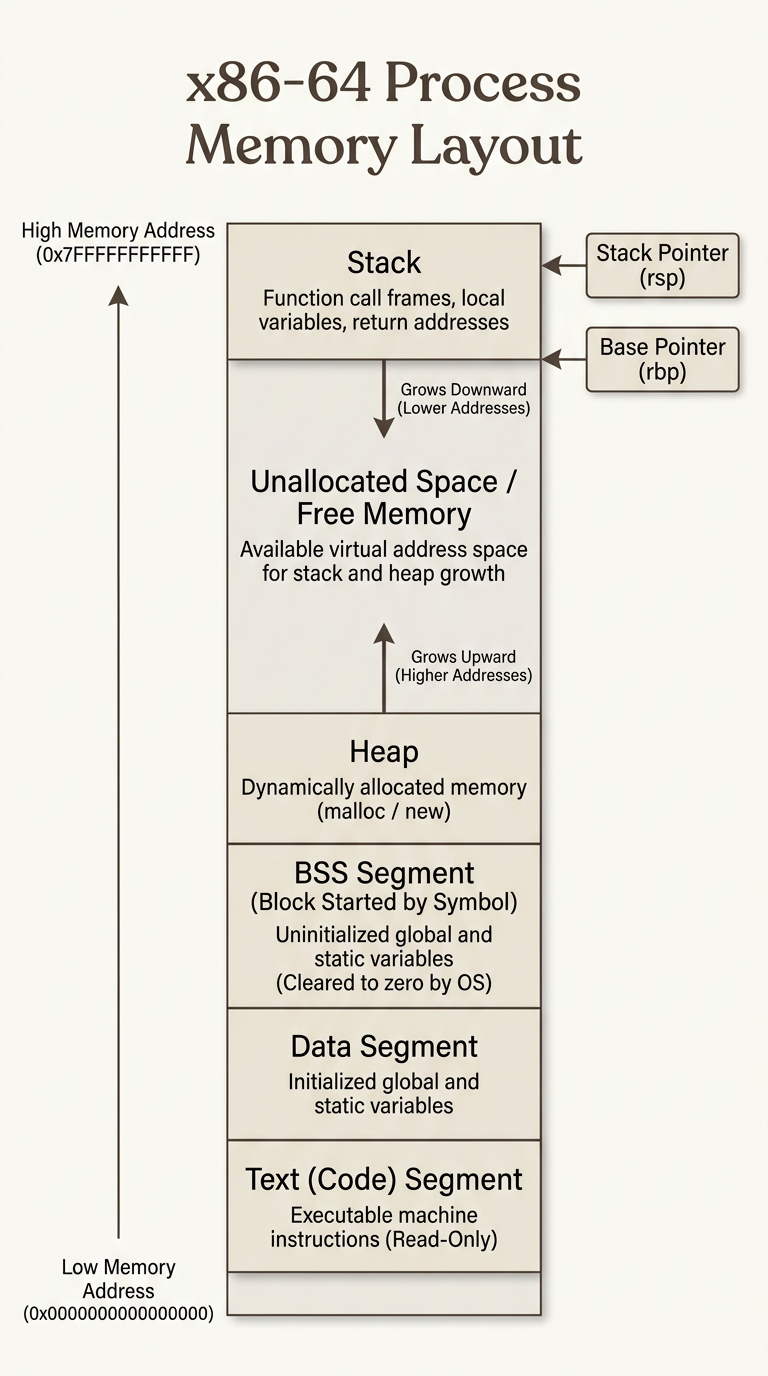
I am initiating a diagram generation to show you how these segments sit in physical and virtual memory. Notice how the Heap and Stack are placed on opposite ends of the unallocated memory pool, growing directly toward each other.

This opposing growth design is an elegant architectural choice. If the Heap and Stack grew in the same direction, one would quickly collide with the other, requiring constant resizing of segment boundaries. By growing towards each other from opposite poles, they maximize the utilization of the available free memory space in the middle.

Let's check your architectural understanding of this layout. If a program experiences a runaway recursion bug where functions continuously call themselves without returning, which boundary condition will occur first in this memory layout?

Which boundary condition occurs first if a program experiences an infinite recursion bug?

You are exactly right. The stack resides at the very top of the virtual address space and grows downward. In the event of a runaway recursion loop, the stack pointer moves lower with every nested call frame until it breaks out of its allocated boundary, colliding with the heap or triggering a page fault that the operating system intercepts as a stack overflow.

The x86-64 Syscall Calling Convention

• Syscall Number: Loaded into rax. This unique integer tells the kernel which service to run (for example, 0 is for read, 1 is for write, and 60 is for exit).
• Arguments: System call arguments are passed in a strict, ordered sequence of registers: rdi (1st argument), rsi (2nd), rdx (3rd), r10 (4th), r8 (5th), and r9 (6th).
• Return Value: Once the kernel finishes, control returns to your program, and the result of the system call is stored in rax. If the value in rax is negative, it typically represents an error code.

; A clean exit system call in x86-64 Linux assembly
mov rax, 60         ; Syscall number 60 is sys_exit
mov rdi, 0          ; Argument 1: Exit code 0 (success)
syscall             ; Invoke the kernel to terminate the program

Let's test your understanding of how these registers transfer control to the kernel during system operations.

Suppose you are writing a routine to print a diagnostic message to the console on Linux. The system call number for sys_write is 1, standard output (stdout) is file descriptor 1, and your buffer pointer and text length are ready. How should you set up your registers before invoking the syscall?