Why do supply chains fail?

To understand why supply chains fail, we first need to map out how they are structured and see how their different parts connect.

Your path

Information Distortion & Bullwhip Effect

Physical Bottlenecks & Operational Failures

External Shocks & Vulnerability

Building Resilient Supply Chains

This learning path is designed to take us from the absolute basics of how a supply chain is put together all the way to how companies build resilience against global crises. Before we dive into our first topic, I want to make sure this path aligns with what you want to get out of our time together.

Are you exploring this for work/studies, or purely out of general curiosity? And how familiar are you already with basic business concepts?

I'm exploring for my studies and have some basic business knowledge.

It is wonderful to hear that you are approaching this from an academic perspective with some business background. Let us examine our plan of study to make sure we are aligned.

Your path

Information Distortion & Bullwhip Effect

Physical Bottlenecks & Operational Failures

External Shocks & Vulnerability

Building Resilient Supply Chains

We will begin with our first focus area, Foundations of Supply Chain Dynamics. Our goal here is to establish a solid baseline by examining what a supply chain actually is, how its individual parts rely on each other, and how the entire system strives to balance supply and demand.

Does this feel like the right starting point for your studies, or would you like to adjust any part of this outline before we begin?

Continue: Let's start with the foundations!

A supply chain is not just a collection of trucks and warehouses; it is a complex, dynamic network designed to bring a product from its raw beginnings straight to the consumer. In academic terms, we define a supply chain as a integrated system of organizations, people, activities, information, and resources that connects to end-customer delivery.

To understand how these networks succeed or fail, we must look at them through the lens of , which views the entire supply chain as a web of highly interdependent parts rather than isolated departments. Within this system, three primary flows keep the network alive:

Physical Flows: The movement of tangible materials and finished goods from suppliers to manufacturers, distributors, retailers, and finally, the consumer.
Information Flows: The transmission of demand signals, order statuses, forecasts, and coordination data across all partners.
Financial Capital Flows: The movement of payments, credit terms, and financial transactions running in the opposite direction, from the paying customer back to the original suppliers.

At its heart, the core operational goal of any supply chain is balancing supply capacity with volatile consumer demand. If supply and demand are misaligned, companies face severe penalties: either excess inventory that drains financial capital, or painful stockouts that drive frustrated customers to competitors.

Explain the difference between physical and informational flows with a real-world example.

To understand the difference between physical and informational flows, we can look at the launch of a high-demand device like a new . The way these two flows interact determines whether the launch is a global success or an expensive failure.

Let us break down how this works in practice during a product rollout:

Physical Flow (Downstream): This is the movement of actual physical assets. It begins with raw lithium and silicon mined from the earth, which are shipped to component factories, assembled into phones in manufacturing plants, loaded onto cargo planes, sorted in distribution centers, and finally placed on retail shelves.
Information Flow (Upstream and Downstream): This is the digital lifeblood of the network. When a customer pre-orders a phone online, that demand signal instantly travels upstream to the retailer, the distributor, the assembly plant, and all the way back to the chip manufacturers. Information flows also move downstream, such as when a shipping carrier sends real-time GPS tracking coordinates to the retailer so they know exactly when the delivery truck will arrive.

In a healthy system, these flows act like a synchronized dance. The information flow predicts and coordinates, while the physical flow executes and delivers.

Operational failures happen when these two flows become mismatched. If a retailer's digital system falsely reports that a warehouse is fully stocked (an information error), but the physical shelves are actually empty, the system will stop ordering shipments. This leads to a severe stockout. Conversely, if demand data is lagged or distorted, a factory might overproduce thousands of devices. This leads to massive physical stockpiles that clog warehouses and tie up millions of dollars in unsold inventory. This breakdown of coordination is a primary driver behind major .

To visualize these parallel dynamics, let us generate a structural diagram of how these physical and informational elements move through the network.

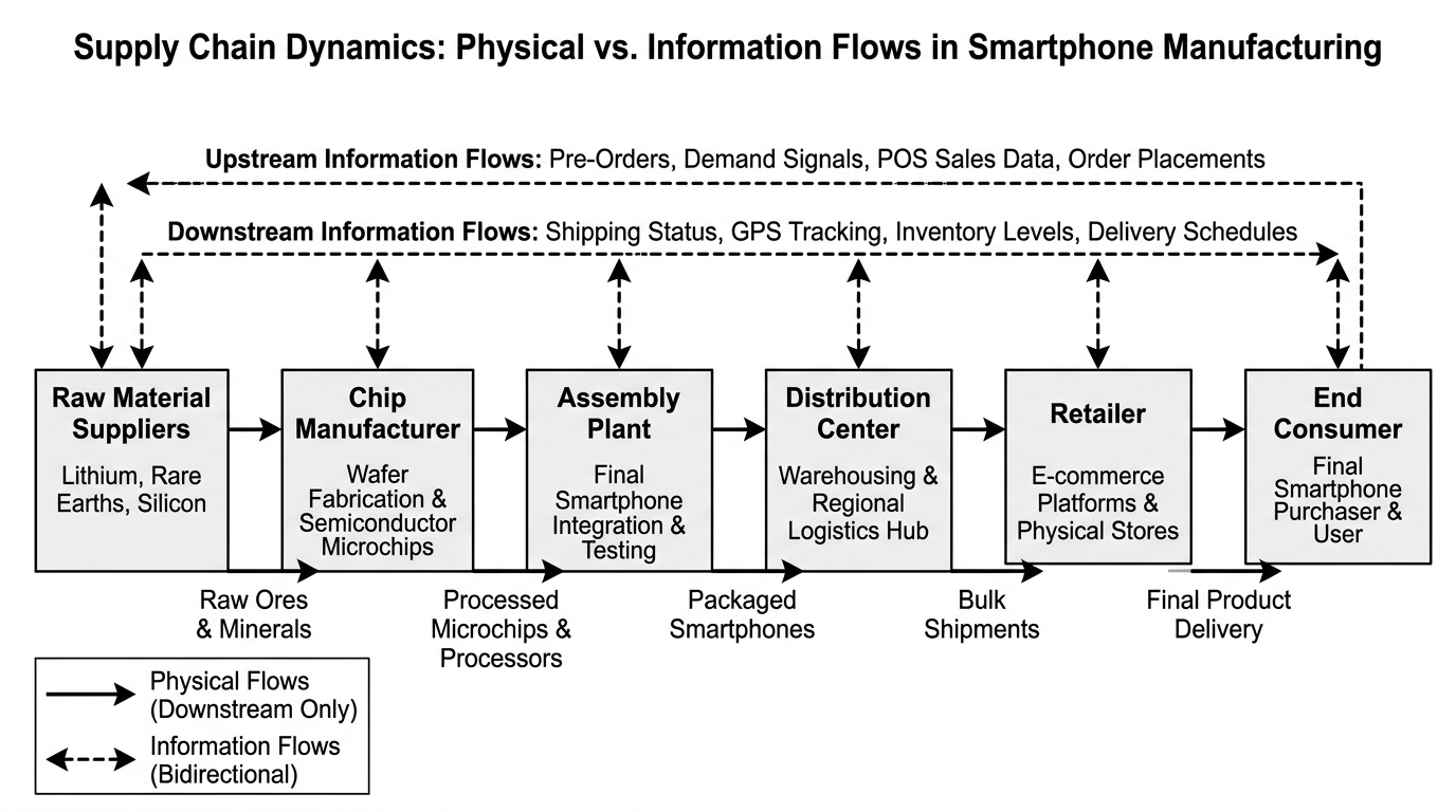
Supply Chain Dynamics: Physical vs. Information Flows in Smartphone ManufacturingDiagram

This diagram highlights how data must travel backward to trigger the forward movement of physical inventory. Now that we have seen how these two flows interact, we can explore what happens when information gets distorted as it travels up the chain. This phenomenon is known as the bullwhip effect.

Would you like to explore how the bullwhip effect distorts these flows, or would you prefer to test your understanding of physical versus informational flows first?

What causes the communication lag between these flows?

The communication lag between physical and informational flows is rarely caused by a single system outage. Instead, it is built directly into how traditional businesses operate and share data across their networks. In academic research, we trace these lags to several root operational causes:

Batch Processing: Many companies do not update their inventory or sales records in real time. Instead, they rely on periodic batch processing, where orders or inventory levels are grouped and processed only once a day, once a week, or even once a month.
Information Silos: Departments within the same company, and separate partners across the supply chain, often operate on incompatible platforms. When systems cannot talk to each other, data must be manually extracted, reformatted, and emailed, which stops real-time visibility.
System Latency and Human Delay: Even when data is available, decision-making latency occurs. Managers must analyze reports, negotiate pricing, verify warehouse capacities, and manually approve purchase orders, adding days or weeks of administrative delay before a physical order is placed.

These communication lags have a direct, damaging effect on operational planning. When demand signals are delayed, upstream partners (like manufacturers and raw material suppliers) are forced to base their production schedules on rather than live customer demand. Because they are operating in the dark, these upstream partners experience extreme planning distortion. By the time a sudden surge in consumer demand finally travels up the chain to the manufacturer, the delay has already caused a stockout. To compensate, partners over-order to build a buffer, which triggers severe demand signal distortion and inventory imbalances across the network.

These lagged communication cycles and distorted planning signals are the direct triggers of the bullwhip effect, which we will study next.

Would you like to explore how this distortion amplifies as it travels further upstream, or would you prefer to test your understanding of supply chain flows with a quick quiz first?

Explain the bullwhip effect with a simple analogy.

To visualize the bullwhip effect, imagine a person holding a long in their hand. If they perform a tiny, sharp snap of their wrist, that small movement creates a modest wave near the handle. As that wave travels down the length of the whip, however, it gathers momentum, amplifying dramatically until the very tip of the whip cracks violently through the air at supersonic speed.

In a supply chain, your hand represents the end customer, and the tip of the whip represents the raw material supplier. Let us look at how a minor fluctuation at the retail level cascades into chaos upstream:

The Customer (The Hand): A retail store normally sells 100 boxes of a popular organic tea each week. Suddenly, due to a minor cold weather spike, sales increase to 110 boxes. This is a tiny 10% bump in actual consumer demand.
The Retailer (The Handle): The store manager notices the increase. Fearing a stockout next week, and wanting to build a , they do not order just 110 boxes from the distributor. Instead, they play it safe and order 125 boxes.
The Distributor (The Middle of the Whip): The distributor sees an order for 125 boxes. They also want to be safe, protect their service levels, and take advantage of bulk shipping discounts. They place an order to the manufacturer for 150 boxes.
The Manufacturer (The Tip of the Whip): Seeing a sudden jump to 150 boxes, the factory manager assumes a major market boom is underway. To ensure they have enough capacity, they order enough raw tea leaves from agricultural suppliers to produce 200 boxes.

Because of a tiny, temporary 10-box shift in real consumer demand, the upstream supplier is suddenly hit with a massive, artificial demand signal for 200 boxes. This leads to extreme overproduction, bloated warehouses, and massive financial waste once the cold snap passes and retail demand returns to normal.

Now that we have explored this classic supply chain phenomenon, we can move forward.

Would you like to explore the core operational strategies companies use to tame the bullwhip effect, or would you prefer to take a quick multiple-choice quiz to test your knowledge on supply chain dynamics first?

How do companies use technology to stop the whip from cracking?

To stop the whip from cracking, companies must replace isolated guesses with shared, real-time data. Modern businesses use integrated technological solutions to bridge the gap between physical and informational flows, ensuring every partner along the chain operates on the exact same demand signals.

These technological solutions target the core drivers of communication lags through several primary systems:

Real-Time POS Data Sharing: Retailers share live data directly with upstream manufacturers. Instead of waiting for weekly order batches, a factory instantly sees when a customer purchases a single item, keeping production tightly aligned with real-world consumption.
Electronic Data Interchange (EDI): This technology standardizes and automates the transmission of structured business documents, such as purchase orders and invoices, between different organizations. EDI eliminates manual email delays and ensures administrative data moves instantly across company borders.
Vendor-Managed Inventory (VMI): In a VMI partnership, the manufacturer takes over the responsibility of managing inventory levels at the retailer's warehouse or distribution center. Guided by shared data, the supplier determines when to replenish stock, eliminating the retailer's tendency to over-order safety stock.
Cloud ERP Integration: By migrating from siloed, legacy databases to unified, cloud-based networks, every partner in the chain gains a single, real-time version of the truth, completely dismantling operational information silos.

When these technologies are integrated, they synchronize the supply chain's physical and informational flows. Automated demand forecasting software can analyze this incoming data stream, stripping away the artificial demand spikes created by panicking middle managers and allowing the entire network to run smoothly. We have completed our exploration of how information distortion and the bullwhip effect can threaten supply chain stability. Before we move on to our next topic, where we will examine physical bottlenecks and operational failures at key nodes like ports and warehouses, let us verify our understanding of these concepts. Are you ready to test your knowledge on the bullwhip effect and these tech solutions with a quick quiz?

In a vendor-managed inventory (VMI) arrangement, how is the bullwhip effect minimized?

Information Distortion & Bullwhip Effect

That is correct. In a vendor-managed inventory setup, the manufacturer bypasses the retailer's inflated safety orders by looking directly at the . This shared visibility stops the demand signal from distorting as it moves upstream.

Your path

External Shocks & Vulnerability

Building Resilient Supply Chains

Now we move into our next focus area: Physical Bottlenecks & Operational Failures. We are shifting our attention from informational errors to the hard, physical constraints that limit how quickly goods can move through a network.

In supply chain design, every physical facility has a maximum operational capacity limit. When the volume of physical goods exceeds this threshold, a bottleneck occurs. Unlike the digital lags we studied earlier, physical bottlenecks are governed by real-world limitations: the number of physical at a warehouse, the square footage of a terminal, or the number of cranes operating at a port.

Consider global maritime ports. A port's capacity is constrained by its channel depth, the speed of its gantry cranes, and the physical space available to stack steel cargo containers. If a fleet of massive container ships arrives simultaneously, a queue forms in the open ocean. This creates a severe congestion bottleneck that delays delivery schedules for weeks downstream.

Would you like to examine what happens when these capacity limits are pushed to the brink, or would you prefer to explore how labor shortages trigger these operational failures first?

How do warehouse capacity limits differ from port limits?

While both warehouse and port capacity limits create physical bottlenecks, they differ fundamentally in their operational environments and the specific variables that restrict their maximum throughput.

Let us contrast the physical constraints of these two vital nodes:

Warehouse Capacity Limits: Inside a warehouse, bottlenecks are dictated by internal storage square footage, the height of the racking systems, the number of physical available for trucks, and the processing speeds of sorting and picking automation. A warehouse bottleneck is primarily a storage and internal sorting constraint.
Port Capacity Limits: Maritime ports are governed by a far more complex set of marine and terrestrial constraints. A port's maximum throughput is limited by (which dictates the size of vessel that can physically enter), the number of massive gantry cranes available to lift containers off ships, vessel berthing space at the docks, and the holding capacity of the container yard.

When a warehouse fills up, it slows down local shipping. When a port hits its limit, it forces massive ships to queue in the ocean, creating a regional transport crisis.

To explore how these physical bottlenecks directly impact shipping timelines and costs across the globe, we can dive deeper into how long delays ripple out from these key nodes.

How do port delays increase overall shipping costs?

When physical bottlenecks clog critical infrastructure nodes like maritime ports, the financial consequences go far beyond simple transit delays. Port congestion triggers a cascading cycle of expenses that directly escalate overall for every player in the network.

These escalating expenses stem from several distinct operational and contractual penalties:

Demurrage and Detention Fees: Ocean carriers charge steep daily penalties when cargo containers sit too long. is charged for containers left inside the port terminal past the allowed free days, while detention is charged for holding onto the physical container equipment outside of the port.
Working Capital Costs: When goods are trapped on container ships waiting in the harbor, a company's financial capital is completely frozen. This inventory is paid for but cannot be sold, which ties up valuable working capital and harms corporate liquidity.
Expedited Freight Rerouting: To avoid missing critical retail windows or halting factory assembly lines, desperate supply chain managers often bypass ocean delays entirely by paying premium rates to via air freight, which can cost up to ten times more than standard sea transit.

These compounding financial strains demonstrate that a physical bottleneck does not just slow down delivery; it directly drains cash reserves and introduces severe volatility into corporate budgets.

Would you like to examine how labor shortages at these ports further trigger these operational bottlenecks, or would you prefer to take a quick multiple-choice quiz to test your understanding of port versus warehouse constraints?

How do port labor shortages worsen these bottlenecks?

When labor shortages strike, they starve these physical nodes of the human capacity required to process goods. A maritime port or cargo terminal cannot run on automated systems alone; it relies heavily on specialized labor like , dockworkers, and drayage truck drivers to maintain its operational pace.

Without sufficient personnel, the operational impact on throughput is immediate and severe, compounding existing bottlenecks in several ways:

Prolonged Vessel Turnaround Times: When dockworker crews are understaffed, lifting containers off a ship takes twice as long. Ships are forced to sit at the berth for days instead of hours, which prevents subsequent vessels from docking and forces them to queue in the open ocean.
Container Yard Congestion: If there is a shortage of yard-hostler drivers, containers pile up at the docks instead of being moved to sorting zones. This physical clutter prevents cranes from dropping off new containers, halting unloading operations entirely.
The Drayage Trucking Bottleneck: Even if a container is unloaded, a shortage of local truck drivers means cargo sits idle on chassis. This lack of prevents goods from leaving the terminal gate, turning the port into an expensive storage lot.

This labor friction turns a temporary delay into a prolonged operational standstill. Now that we have analyzed how labor shortages aggravate physical bottlenecks, we can look at how physical assets become vulnerable to geographical and single-source constraints.

Would you like to examine single points of failure in global sourcing and transport, or would you prefer to test your knowledge of labor's role in port capacity first?

What are some real examples of major port labor strikes?

When labor negotiations stall and dockworkers walk out, the flow of goods does not just slow down; it stops completely. Two of the most significant in United States history illustrate how quickly labor disputes can paralyze port throughput and freeze regional supply chains: the 2002 West Coast Port Lockout and the 2024 International Longshoremen's Association (ILA) East and Gulf Coast Strike.

Let us examine the operational realities and structural damage caused by these two major labor disputes:

The 2002 West Coast Port Lockout: Following a contract dispute over the introduction of barcode scanners and tracking technology, employers locked out members of the International Longshore and Warehouse Union (ILWU). This dispute shuttered 29 major ports from Seattle to San Diego for 10 days, trapping over 200 cargo ships at sea and costing the U.S. economy an estimated $1 billion per day.
The 2024 ILA East and Gulf Coast Strike: In October 2024, the ILA launched a strike that shut down 36 container ports from Maine to Texas. The union demanded wage increases and a complete ban on the . Even though the strike lasted only three days, it created a massive backlog of container ships in the Atlantic Ocean, requiring nearly a month of backlogged recovery work for every single day of the strike.

These events prove that labor disputes do not just delay local deliveries; they completely block the gateways of trade, triggering cascading physical bottlenecks that take weeks to resolve.

This complete halt of port operations shows that physical networks are only as strong as their most vulnerable nodes.

Now that we have analyzed how labor strikes paralyze key gateways, we can move forward to the final element of this topic: identifying critical single points of failure in global sourcing and transit.

Would you like to explore geographical chokepoints and single-source supplier vulnerabilities, or would you prefer to test your understanding of port labor dynamics with a quick multiple-choice quiz first?

What are the most vulnerable geographical chokepoints in the world?

When we study the physical network of global trade, we see that it is not a uniform, open web. Instead, it is highly concentrated. The vast majority of international maritime commerce must squeeze through a handful of narrow, highly vulnerable geographic corridors known as .

Let us examine the three most critical chokepoints that keep global supply chain planners up at night:

The Suez Canal (Egypt): Connecting the Mediterranean Sea to the Red Sea, this narrow artificial waterway handles roughly 12% of all global trade. It serves as the primary maritime shortcut between Asia and Europe, eliminating the need to sail around the entire African continent.
The Strait of Malacca (Southeast Asia): Positioning itself between the Malay Peninsula and Sumatra, this 550-mile-long channel is the primary shipping lane linking the Indian Ocean with the Pacific Ocean. It is the busiest chokepoint in the world, carrying over 25% of all sea-borne trade, including key energy supplies traveling to East Asian markets.
The Panama Canal (Panama): Cutting through the Isthmus of Panama, this lock-based canal connects the Atlantic and Pacific Oceans. It is a critical gateway for trade between East Asia and the US East Coast. Unlike the other sea lanes, its capacity is strictly governed by needed to operate its massive lock systems.

The absolute fragility of these corridors was vividly demonstrated during the , when a single ultra-large container ship, the Ever Given, ran aground in a sandstorm. For six days, the ship completely wedged itself across the canal, blocking over 350 vessels behind it. This single physical failure stranded nearly $10 billion in daily cargo, disrupted global manufacturing schedules, and caused shipping rates to spike worldwide, proving that a bottleneck at a single node can instantly paralyze the entire global network.

To understand the spatial relationships between these global chokepoints and how they shape international trade routes, let us explore an interactive map of these critical maritime channels.

Primary Global Maritime Chokepoints

Interactive map loads after page hydration.

Open this location in Apple Maps

Map highlighting the Suez Canal, Strait of Malacca, and Panama Canal—the three primary chokepoints that dictate global shipping lanes.

This map shows how highly concentrated international shipping corridors are, making them vulnerable to localized physical disruptions. Alongside geographical chokepoints, companies must also guard against the operational risk of relying on a for critical components, which can create a single point of failure within their upstream sourcing network.

We have completed our exploration of our current focus area: Physical Bottlenecks & Operational Failures. We have analyzed how physical capacity limits, labor shortages, geographic chokepoints, and supplier dependencies can restrict the flow of goods and escalate costs across the network.

Would you like to test your understanding of these physical constraints with a quick multiple-choice quiz, or should we continue directly to our next focus area, External Shocks & Vulnerability?

Continue to the next focus area: External Shocks & Vulnerability.

Now we enter our fourth focus area, External Shocks & Vulnerability, shifting our focus from localized operational failures to massive, unpredictable forces that strike from the outside. In academic supply chain theory, an is defined as an unexpected, exogenous event that originates outside the network but severely disrupts the internal flow of goods, information, and capital. These shocks are highly systemic, meaning they rarely remain confined to a single node and instead trigger a across the entire global network.

To analyze how these unpredictable forces destabilize global networks, we categorize external shocks into three primary, high-impact domains:

Geopolitical Disruptions: Wars, regional conflicts, trade disputes, and sudden (like tariffs or trade sanctions) can instantly close off entire geographic corridors or render key suppliers inaccessible.
Environmental Shocks: Natural disasters, extreme weather events, and climate-induced disruptions physically destroy infrastructure, halt manufacturing plants, and block transport routes.
Cybersecurity and Digital Failures: As supply chains become increasingly digitized, malware attacks, software glitches, and cloud outages can paralyze the information flows that coordinate physical logistics, halting operations just as effectively as a physical roadblock.

To ground these concepts, let us look at how geopolitical conflicts actively disrupt global commerce. Consider the Russia-Ukraine War: beyond the tragic human toll, the conflict instantly choked off key agricultural exports like wheat and fertilizer, and triggered severe by disrupting oil and natural gas flows. Similarly, growing trade tensions and tariff disputes between major economic superpowers force high-tech companies to continuously scramble and split their sourcing operations to avoid crippling financial penalties.

These geopolitical disruptions show that global networks remain highly sensitive to regional political stability.

Would you like to examine how natural disasters and extreme climate events physically paralyze logistics, or would you prefer to test your understanding of geopolitical shocks with a quick multiple-choice quiz first?

Continue to environmental and climate-induced disruptions.

While geopolitical friction redraws trade routes on a map, environmental shocks physically dismantle the infrastructure supporting them. present a unique operational challenge because they are completely non-negotiable; you cannot negotiate with a hurricane or draft a contract to bypass a drought.

These climate-induced crises disrupt physical flows through several distinct environmental mechanisms:

Infrastructure Destruction: Superstorms and earthquakes do not just cause delays; they physically erase critical nodes. , like hurricanes, can collapse gantry cranes at ports, flood coastal warehouses, and completely wash away highway networks, halting regional logistics for months.
Transport Route Closures: Inland waterways are highly sensitive to weather variations. For instance, when severe summer droughts hit Europe, major rivers like the Rhine dry up, preventing cargo barges from sailing and forcing freight onto already-congested rail lines.
Agricultural and Commodity Shocks: Freezes, droughts, and floods can instantly wipe out regional harvests. A severe crop failure in one region triggers immediate global ingredient shortages, driving up raw material costs and forcing manufacturers to rapidly seek alternative sources.

To ground this in academic theory, we can look at the 2011 Thailand Floods. Thailand produces a massive portion of the world's . When heavy monsoon rains flooded industrial parks, production ground to a halt. This single environmental shock caused a global shortage of computer storage, doubling market prices and stalling assembly lines at electronics giants worldwide.

Now that we have analyzed how environmental forces physically paralyze logistics, we have only one remaining threat area to explore under external shocks: the vulnerabilities of our digital infrastructure. Would you like to examine how cyberattacks and software glitches trigger massive digital supply chain failures, or would you prefer to test your understanding of environmental disruptions with a quick multiple-choice quiz first?

Continue to cybersecurity and digital infrastructure vulnerabilities.

Our physical logistics networks are held together by invisible digital threads. As supply chains have digitized to combat communication lags, they have inadvertently exposed themselves to a new breed of vulnerability: . When the software, cloud networks, or cybersecurity defenses of a key node collapse, the physical movement of cargo stops just as abruptly as if a port had been locked down by a strike.

We analyze these modern, high-impact digital threats through three primary operational vectors:

Targeted Cyberattacks: Malicious actors deploy ransomware to lock down the operating systems of shipping giants, port terminals, and distributors, demanding multi-million dollar payouts to restore access to critical shipping manifests and route planning software.
Software Update Glitches: The complex interdependence of modern business networks means that a single flawed security update can paralyze global commerce. A prime example is the 2024 CrowdStrike incident, where a faulty software update triggered a massive blue-screen outage across millions of Windows devices. This digital failure grounded cargo flights, froze port terminal operating systems, and disrupted logistics networks globally.
Cloud Outages and Concentration Risk: Because thousands of logistics companies, customs agencies, and third-party warehouse providers rely on the exact same handful of public cloud platforms, a single server farm outage can trigger a , leaving supply chain managers completely blind to their inventory positions.

This susceptibility to digital collapses shows that modern supply chains are highly vulnerable to both physical and technological disruptions.

We have completed our comprehensive study of External Shocks & Vulnerability. We have analyzed how unpredictable external forces—ranging from regional wars and extreme climate events to global software glitches—can instantly paralyze trade flows.

Now, we are ready to move on to our fifth and final focus area: Building Resilient Supply Chains, where we will transition from analyzing why networks fail to discovering how companies actively design systems to survive these shocks.

Let us display the learning path to visualize our progress as we step into this final area of study.

Your path

Building Resilient Supply Chains

In this final focus area, we will examine how modern enterprises balance the cost-efficiencies of lean inventory with the security of operational resilience. To kickstart this discussion, would you like to explore the strategic trade-offs between safety stock and just-in-time inventory systems, or would you prefer to test your understanding of cybersecurity and digital failures with a quick multiple-choice quiz first?

Why is the trade-off between safety stock and just-in-time so difficult?

The trade-off between safety stock and just-in-time (JIT) systems is difficult because it represents a fundamental clash between operational cost-efficiency and supply chain survival. At its core, this tension forces companies to choose between the high financial penalties of holding excess inventory and the devastating risks of failing to meet customer demand.

To understand why this is a continuous tightrope walk for supply chain managers, let us analyze the operational mechanics of both extremes:

The Lean Efficiency of Just-In-Time (JIT): Pioneered in automotive manufacturing, JIT aims to minimize waste by keeping inventory levels as close to zero as possible. Under JIT, parts and raw materials arrive at the factory floor exactly when they are needed for production. This frees up massive amounts of working capital and eliminates .
The Protective Cushion of Safety Stock: Also known as Just-In-Case (JIC), this strategy maintains buffer inventory to protect against sudden demand surges or upstream delays. While this ensures order fulfillment, it ties up cash reserves, increases warehouse renting expenses, and risks product obsolescence.

When a company leans too far toward JIT to maximize short-term profits, it leaves itself completely exposed to external shocks. A classic historical example of a JIT failure occurred at . By operating on a highly conservative, lean inventory strategy, Apple was caught completely unprepared when orders spiked for its new Power Macintosh systems. Lacking safety stock, they could not fulfill the demand, which resulted in lost market share and severe reputational damage.

This illustrates that while JIT works beautifully during times of absolute stability, any physical, digital, or environmental disruption instantly triggers a . When a stockout occurs, a business does not just lose an immediate sale; it suffers a long-term erosion of customer goodwill, as frustrated buyers quickly migrate to competitors who kept buffers in place.

Finding the sweet spot between these two models requires sophisticated calculation and risk assessment. To explore how companies actively balance these variables, would you like to look at how businesses calculate their optimal safety stock levels, or would you prefer to see how hybrid models like dual-sourcing are used to bridge the gap between JIT and safety buffers?

How do companies calculate optimal safety stock levels?

Calculating optimal safety stock levels is not a matter of guesswork; it relies on mathematical modeling designed to absorb statistical variance. To achieve this, companies must first establish a , which represents the desired probability of not running out of stock during a lead time cycle. This target is then combined with the statistical variability of both customer demand and supplier delivery times to determine the precise buffer required.

To calculate this mathematically, supply chain planners use the classic safety stock formula, which isolates and accounts for key operational variables:

SS = Z \times \sqrt{L \sigma_d^2 + d^2 \sigma_L^2}

This formula highlights how safety stock acts as an insurance policy. If your customer demand is perfectly stable (

\sigma_d = 0

) and your supplier is perfectly reliable (

\sigma_L = 0

), the formula drops to zero, and you can operate a pure system. However, in reality, variability exists on both sides, and this formula quantifies exactly how much physical inventory is needed to insulate the business from those real-world fluctuations.

To contrast how these buffer calculations change the way companies place day-to-day replenishment orders, let us compare safety stock formulas directly with JIT reorder point models. We can look at this comparison in a structured table.

Operational Metric	Safety Stock Model (Just-In-Case)	Reorder Point Model (Just-In-Time)
Primary Objective	Protect against unexpected variability in demand and supply	Replenish inventory exactly as it is depleted to maintain a lean flow
Inventory Level	Maintained as a constant minimum buffer (never intended to be used in normal operations)	Declines toward zero, triggering a replacement order just in time
Calculation Focus	Accounts for statistical variance ( $\sigma_d$ and $\sigma_L$ ) and service level targets	Focuses on deterministic averages (Average Lead Time $\times$ Average Daily Demand)
Financial Trade-off	Higher holding costs and capital tied up, but minimal risk of stockouts	Lowest possible holding costs, but extreme vulnerability to any supply disruption

This comparison shows that while safety stock calculations are designed to manage volatility, JIT models assume a high level of predictability. Now that we have analyzed how safety stock is mathematically calculated and contrasted it with lean JIT replenishment, we can explore how companies build modern resilience by combining these models into hybrid networks. Would you like to examine how hybrid models like dual-sourcing, nearshoring, and regional safety buffers are designed to bridge the gap between lean efficiency and security, or would you prefer to test your understanding of safety stock calculations with a quick multiple-choice quiz first?

How does dual-sourcing differ from nearshoring?

While both strategies aim to insulate a business from unexpected supply chain disruptions, dual-sourcing and nearshoring approach risk mitigation from entirely different operational dimensions. is a diversification strategy focused on supplier redundancy, where a company splits its purchasing contracts between two distinct vendors. In contrast, nearshoring is a geographic relocation strategy that moves manufacturing facilities or suppliers closer to the organization's primary consumer market.

To understand how these two strategies compare across key operational variables, we can analyze their differences in geographic focus, risk mitigation, and cost structures:

Geographic Focus: Dual-sourcing does not require changing where your suppliers are located; you can dual-source from two separate factories located in the same country. Nearshoring, however, is fundamentally geographical. It involves bringing your from a distant offshore country (like China) to a nearby nation (such as Mexico for a US-based firm).
Risk Mitigation Profile: Dual-sourcing protects against individual supplier-level failures, like a localized labor strike or a factory-specific machinery breakdown. Nearshoring protects against regional, transit-level shocks. By reducing the physical distance goods must travel, nearshoring bypasses high-seas transit risks, port congestion, and long shipping lead times.
Operational Cost Structure: Dual-sourcing often increases raw material unit costs because splitting your order volume between two suppliers reduces your bulk purchasing power. might also increase labor costs compared to deep offshore regions, but it dramatically lowers international shipping expenses, customs tariffs, and holding costs associated with inventory trapped in transit.

Rather than choosing just one of these methods, many modern enterprises combine them into a powerful hybrid model. For instance, a tech manufacturer might dual-source a critical component by assigning 80% of its volume to a low-cost offshore supplier to maximize efficiency, while assigning 20% to a nearshore supplier to keep a rapid-response channel active in case of an emergency. Now that we have compared dual-sourcing and nearshoring, we can look at how companies design regional safety buffers and build comprehensive, end-to-end network resilience. Would you like to explore how regional safety buffers work in hybrid supply chain models, or would you prefer to test your understanding of dual-sourcing versus nearshoring with a quick multiple-choice quiz first?

Continue to regional safety buffers and hybrid resilience models.

While diversifying your supplier base and shifting locations closer to home are excellent ways to minimize risk, modern supply chains also manage localized spikes in volatility through . Instead of consolidating all safety stock in a single giant, centralized warehouse, companies distribute physical inventory buffers across strategically positioned regional nodes.

This decentralized approach operates as a physical shock absorber. By placing regional warehouses on the consumer side of geographic bottlenecks, companies can guarantee that a sudden ocean freight halt or port shutdown will not instantly starves local retail outlets of product. This brings us directly to the concept of hybrid resilience models.

In academic business theory, a hybrid model does not force a company to choose between the absolute lowest cost of just-in-time and the absolute safety of redundant buffers. Instead, companies construct an integrated matrix. They might apply extreme JIT principles to highly predictable, locally-sourced components, while concurrently maintaining and utilizing dual-sourcing channels for unpredictable, highly critical materials.

To tie these diverse strategies together, we rely on the final tool in our resilience toolkit: end-to-end (E2E) visibility and real-time network intelligence. This technology acts as the digital nervous system of the supply chain. By sharing real-time electronic data across all suppliers, carriers, and retailers, companies can spot a localized disruption the second it occurs, allowing them to dynamically reroute shipments and adjust regional buffer levels before a minor delay cascades into a total network collapse.

This concludes our comprehensive curriculum on Why Supply Chains Fail. We have explored the entire spectrum of supply chain mechanics, from demand signal distortions and physical chokepoints to external digital shocks and modern resilience strategies.

To wrap up this final session, how would you like to proceed?

Explain hybrid resilience with a real-world example

To understand how these concepts operate outside of academic textbooks, we can analyze the real-world strategy of , a pioneer that spent decades perfecting lean, just-in-time (JIT) operations. Following a series of catastrophic disruptions, the automotive giant was forced to completely re-engineer its philosophy, building the modern gold standard for hybrid resilience.

Historically, Toyota operated on a pure JIT model, but the vulnerability of this strategy was brutally exposed during the . The disaster devastated northern Japan, knocking out a single, critical factory belonging to Renesas Electronics—a key supplier that produced over 40% of the global automotive industry's microcontrollers. Because Toyota carried virtually zero safety stock, this single-source failure forced them to halt domestic vehicle assembly lines for weeks, costing them hundreds of thousands of units in lost production and temporarily stripping them of their global market leadership.

In response to this crisis, Toyota did not abandon JIT; instead, they pioneered a highly sophisticated hybrid resilience model based on three core pillars:

The Business Continuity Plan (BCP) Registry: Toyota mapped their entire, multi-tiered supplier network down to the raw material level. They identified roughly 1,500 critical, highly specialized components—such as microchips—that could not be easily replaced.
Strategic Regional Buffers: For those 1,500 vulnerable components, Toyota abandoned pure JIT and mandated that suppliers hold regional safety buffers ranging from two to six months of inventory.
Proactive Dual-Sourcing: They diversified their manufacturing footprint, ensuring that critical components were dual-sourced across different geographic regions to prevent a single local disaster from crippling global production.

When the global semiconductor shortages of 2021 struck, while rival automakers operating on pure JIT models were forced to shutter factories immediately, Toyota's regional safety buffers and supplier visibility kept their production lines humming for months, proving that hybrid resilience is the ultimate competitive shield.

This real-world transition demonstrates that true resilience is not about carrying massive inventory for every single part, but rather about surgically placing safety buffers where they are needed most while maintaining lean operations everywhere else. We have now fully covered our entire curriculum on Why Supply Chains Fail. You have successfully analyzed the entire spectrum of supply chain mechanics, from demand signal distortions and physical chokepoints to external digital shocks and modern hybrid resilience strategies. To wrap up your learning journey, would you like to compile this knowledge with a comprehensive study guide, test your retention with a final quiz, or complete a structured review of the core concepts?

Let us do a quick, structured recap of the major takeaways

We have reached a major milestone. Having navigated the intricate mechanics of global trade, we have completed all five primary focus areas of our curriculum. To cement your mastery, let us perform a structured recap of the critical takeaways from each phase of our journey.

The Journey of Supply Chain Vulnerability & Resilience

Focus Area	Core Concept & Academic Theory	Critical Real-World Takeaway
1. Foundations of Dynamics	The multi-tiered network relies on the synchronized flow of physical goods, information, and financial capital.	Interdependence means that a failure at any single node instantly destabilizes adjacent partners.
2. Information & Bullwhip	Demand signal distortion amplifies upstream due to lagged communication, batch ordering, and decision latency.	Small shifts in consumer demand lead to massive, costly inventory imbalances for raw material suppliers.
3. Physical Bottlenecks	Absolute capacity limits at physical nodes (ports, warehouses) and geographical chokepoints restrict throughput.	Incidents like the Ever Given Suez blockage prove that physical bottlenecks quickly paralyze global trade.
4. External Shocks	Systemic, exogenous disruptions (geopolitical, climate, digital) propagate through the network via ripple effects.	The 2011 Thailand floods and the 2024 CrowdStrike outage show that non-negotiable shocks halt physical operations.
5. Resilient Strategies	Balancing lean cost-efficiencies with strategic buffers, dual-sourcing, nearshoring, and E2E visibility.	Toyota's post-2011 hybrid model demonstrates that targeted regional safety buffers protect operations without sacrificing overall efficiency.

This progression highlights a fundamental truth in modern operations: supply chains do not fail because of isolated events, but because of accumulated blind spots, rigid architectures, and a lack of real-time visibility. By understanding how demand distortions, physical bottlenecks, external shocks, and lean vulnerabilities interact, you can transition from merely managing logistics to actively architecting in a highly volatile global environment.

You have successfully completed the entire learning objective for this course. To wrap up this learning journey, would you like to compile this entire body of knowledge into a comprehensive study guide, or would you prefer to test your retention of these concepts with a final quiz?